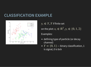
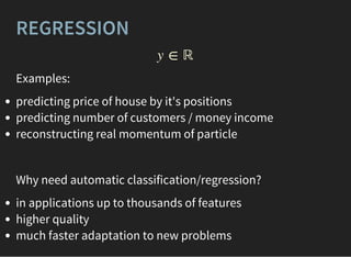
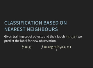
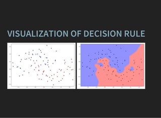
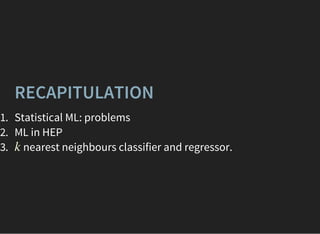
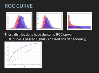
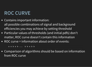
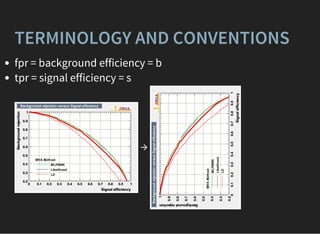
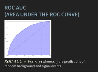
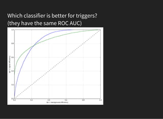
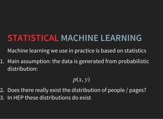
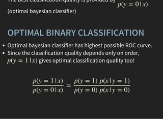
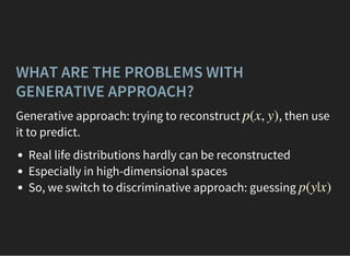
The document presents an introductory lecture on machine learning in high energy physics, covering topics such as the application of machine learning techniques in particle identification, classification, and regression analysis. It discusses concepts like overfitting, nearest neighbors classifiers, and the ROC curve for evaluating classifier performance. The lecture emphasizes the importance of understanding data distributions and highlights various approaches to predictive modeling including Bayesian classifiers and logistic regression.


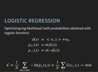
![FINDING OPTIMAL PARAMETERS
A good initial guess: get such , that error of
classification is minimal ([true] = 1, [false] = 0):
Discontinuous optimization (arrrrgh!)
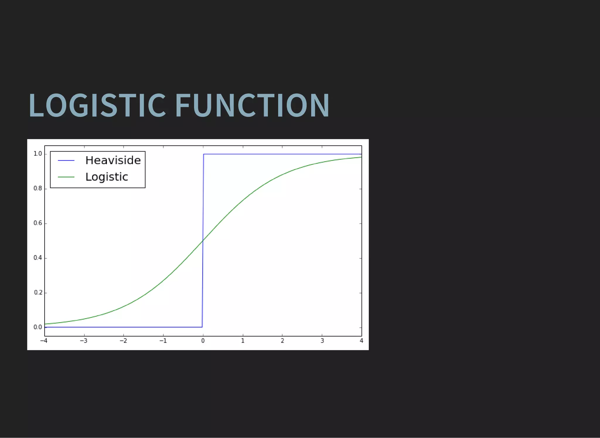
Let's make decision rule smooth
w, w0
= [ ≠ sgn(d( ))]
∑
i∈events
yi xi
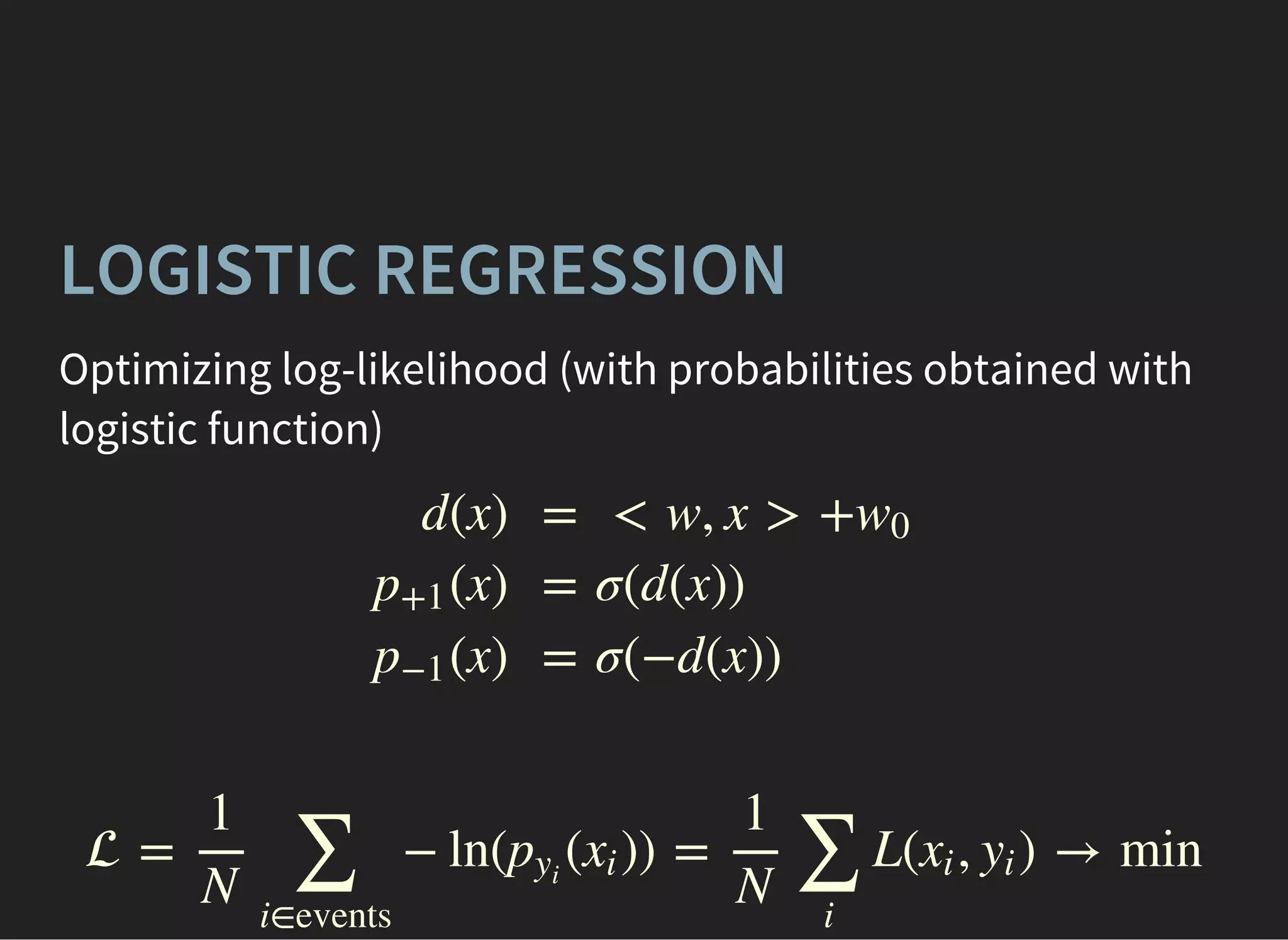
(x)p+1
(x)p−1
= f (d(x))
= 1 − (x)p+1
⎧
⎩
⎨
⎪
⎪
f (0) = 0.5
f (x) > 0.5
f (x) < 0.5
if x > 0
if x < 0](https://image.slidesharecdn.com/lecture1-150907123024-lva1-app6892/85/MLHEP-2015-Introductory-Lecture-1-41-320.jpg)


![FINDING OPTIMAL PARAMETERS
A good initial guess: get such , that error of
classification is minimal ([true] = 1, [false] = 0):
Discontinuous optimization (arrrrgh!)
Let's make decision rule smooth
w, w0
= [ ≠ sgn(d( ))]
∑
i∈events
yi xi
(x)p+1
(x)p−1
= f (d(x))
= 1 − (x)p+1
⎧
⎩
⎨
⎪
⎪
f (0) = 0.5
f (x) > 0.5
f (x) < 0.5
if x > 0
if x < 0](https://image.slidesharecdn.com/lecture1-150907123024-lva1-app6892/75/MLHEP-2015-Introductory-Lecture-1-41-2048.jpg)


![[ppt]](https://cdn.slidesharecdn.com/ss_thumbnails/ppt2931-thumbnail.jpg?width=600ounds&width=560&fit=bounds)
![[ppt]](https://cdn.slidesharecdn.com/ss_thumbnails/ppt3441-thumbnail.jpg?width=600ounds&width=560&fit=bounds)


