Module 5_Hashing_part2_Cybersecurity.pptx

Module 5_Hashing_part2_Cybersecurity.pptx

• 1.
  Hashing: Collision ResolutionSchemes 1 • Collision Resolution Techniques • Separate Chaining • Separate Chaining with String Keys • Separate Chaining versus Open-addressing • The class hierarchy of Hash Tables • Implementation of Separate Chaining • Introduction to Collision Resolution using Open Addressing • Linear Probing
• 2.
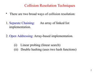
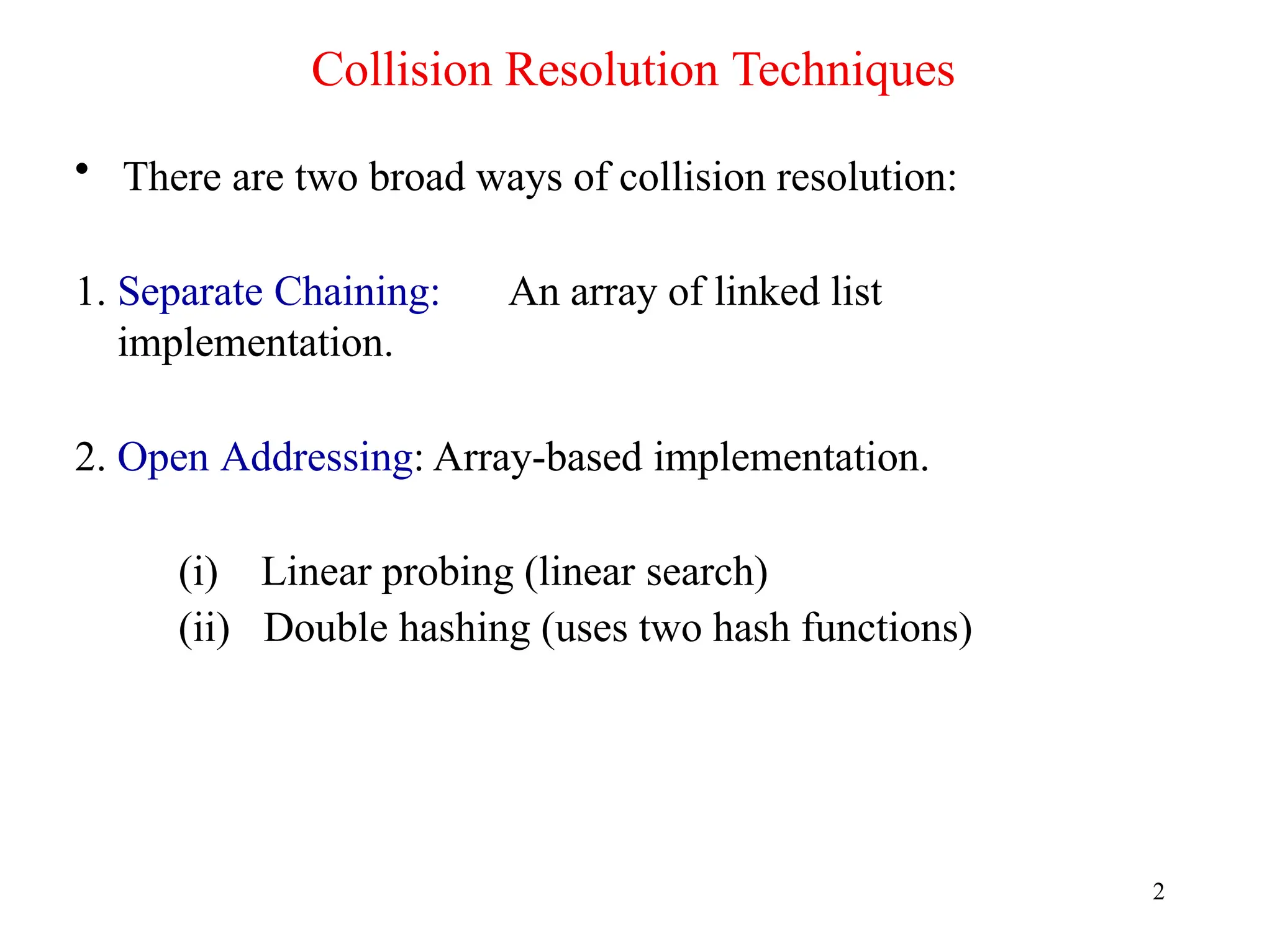
  Collision Resolution Techniques 2 •There are two broad ways of collision resolution: 1. Separate Chaining: An array of linked list implementation. 2. Open Addressing: Array-based implementation. (i) Linear probing (linear search) (ii) Double hashing (uses two hash functions)
• 3.
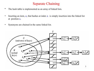
  Separate Chaining • Thehash table is implemented as an array of linked lists. • Inserting an item, r, that hashes at index i is simply insertion into the linked list at position i. • Synonyms are chained in the same linked list. 3
• 4.
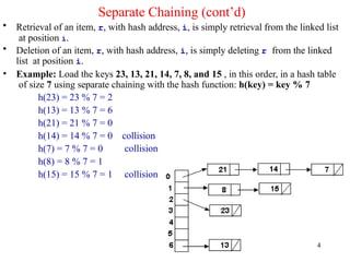
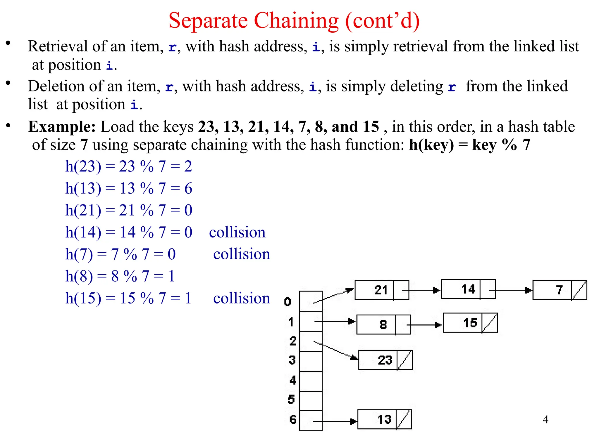
  Separate Chaining (cont’d) •Retrieval of an item, r, with hash address, i, is simply retrieval from the linked list at position i. • Deletion of an item, r, with hash address, i, is simply deleting r from the linked list at position i. • Example: Load the keys 23, 13, 21, 14, 7, 8, and 15 , in this order, in a hash table of size 7 using separate chaining with the hash function: h(key) = key % 7 h(23) = 23 % 7 = 2 h(13) = 13 % 7 = 6 h(21) = 21 % 7 = 0 collision collision h(14) = 14 % 7 = 0 h(7) = 7 % 7 = 0 h(8) = 8 % 7 = 1 h(15) = 15 % 7 = 1 collision 4
• 5.
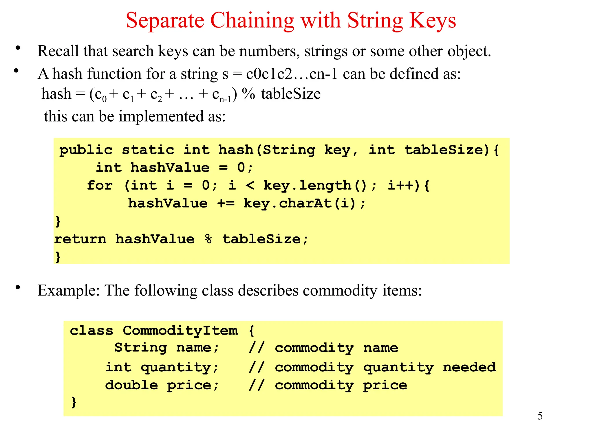
  Separate Chaining withString Keys 5 • Recall that search keys can be numbers, strings or some other object. • A hash function for a string s = c0c1c2…cn-1 can be defined as: hash = (c0 + c1 + c2 + … + cn-1) % tableSize this can be implemented as: • Example: The following class describes commodity items: public static int hash(String key, int tableSize){ int hashValue = 0; for (int i = 0; i < key.length(); i++){ hashValue += key.charAt(i); } return hashValue % tableSize; } class CommodityItem String name; { // commodity name int quantity; // commodity quantity needed double price; } // commodity price
• 6.
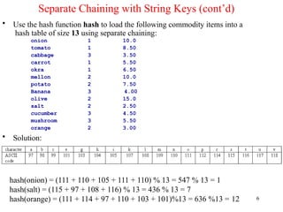
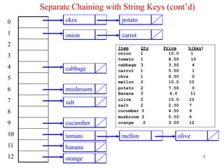
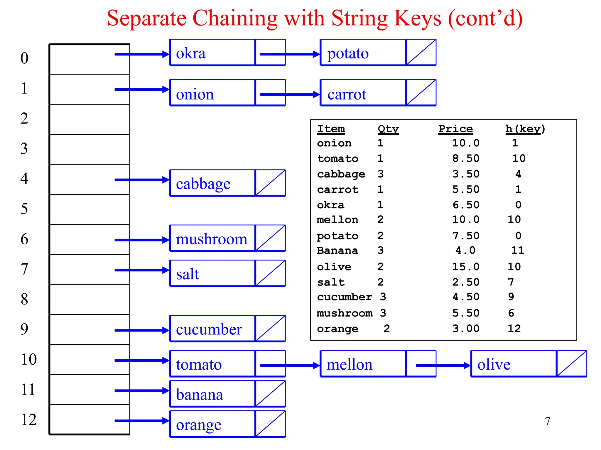
  6 Separate Chaining withString Keys (cont’d) • Use the hash function hash to load the following commodity items into a hash table of size 13 using separate chaining: onion 1 10.0 tomato 1 8.50 cabbage 3 3.50 carrot 1 5.50 okra 1 6.50 mellon 2 10.0 potato 2 7.50 Banana 3 4.00 olive 2 15.0 salt 2 2.50 cucumber 3 4.50 mushroom 3 5.50 orange 2 3.00 • Solution: hash(onion) = (111 + 110 + 105 + 111 + 110) % 13 = 547 % 13 = 1 hash(salt) = (115 + 97 + 108 + 116) % 13 = 436 % 13 = 7 hash(orange) = (111 + 114 + 97 + 110 + 103 + 101)%13 = 636 %13 = 12
• 7.
  7 Separate Chaining withString Keys (cont’d) 0 1 2 3 4 5 6 7 8 9 10 11 12 okra potato onion carrot Item Qty Price h(key) onion 1 10.0 1 tomato 1 8.50 10 cabbage 3 3.50 4 carrot 1 5.50 1 okra 1 6.50 0 mellon 2 10.0 10 potato 2 7.50 0 Banana 3 4.0 11 olive 2 15.0 10 salt 2 2.50 7 cucumber 3 4.50 9 mushroom 3 5.50 6 orange 2 3.00 12 cabbage mushroom salt cucumber mellon banana tomato olive orange
• 8.
  • All itemsare stored in the hash table itself. • In addition to the cell data (if any), each cell keeps one of the three states: EMPTY, OCCUPIED, DELETED. • While inserting, if a collision occurs, alternative cells are tried until an empty cell is found. • Deletion: (lazy deletion): When a key is deleted the slot is marked as DELETED rather than EMPTY otherwise subsequent searches that hash at the deleted cell will fail. • Probe sequence: A probe sequence is the sequence of array indexes that is followed in searching for an empty cell during an insertion, or in searching for a key during find or delete operations. • The most common probe sequences are of the form: hi(key) = [h(key) + c(i)] % n, for i = 0, 1, …, n-1. where h is a hash function and n is the size of the hash table • The function c(i) is required to have the following two properties: Property 1: c(0) = 0 Property 2: The set of values {c(0) % n, c(1) % n, c(2) % n, . . . , c(n-1) % n} must be a permutation of {0, 1, 2,. . ., n – 1}, that is, it must contain every integer between 0 and n - 1 inclusive. 12 Introduction to Open Addressing
• 9.
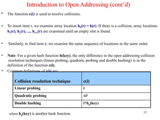
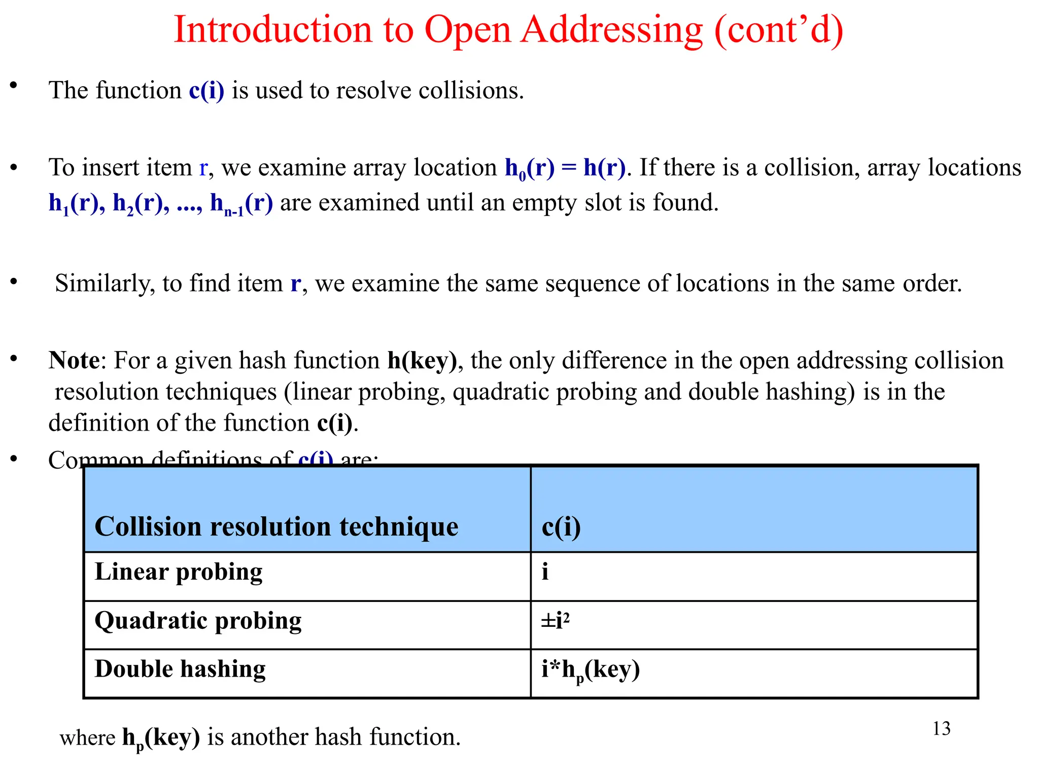
  13 Introduction to OpenAddressing (cont’d) • The function c(i) is used to resolve collisions. • To insert item r, we examine array location h0(r) = h(r). If there is a collision, array locations h1(r), h2(r), ..., hn-1(r) are examined until an empty slot is found. • Similarly, to find item r, we examine the same sequence of locations in the same order. • Note: For a given hash function h(key), the only difference in the open addressing collision resolution techniques (linear probing, quadratic probing and double hashing) is in the definition of the function c(i). • Common definitions of c(i) are: Collision resolution technique c(i) Linear probing i Quadratic probing ±i2 Double hashing i*hp(key) where hp(key) is another hash function.
• 10.
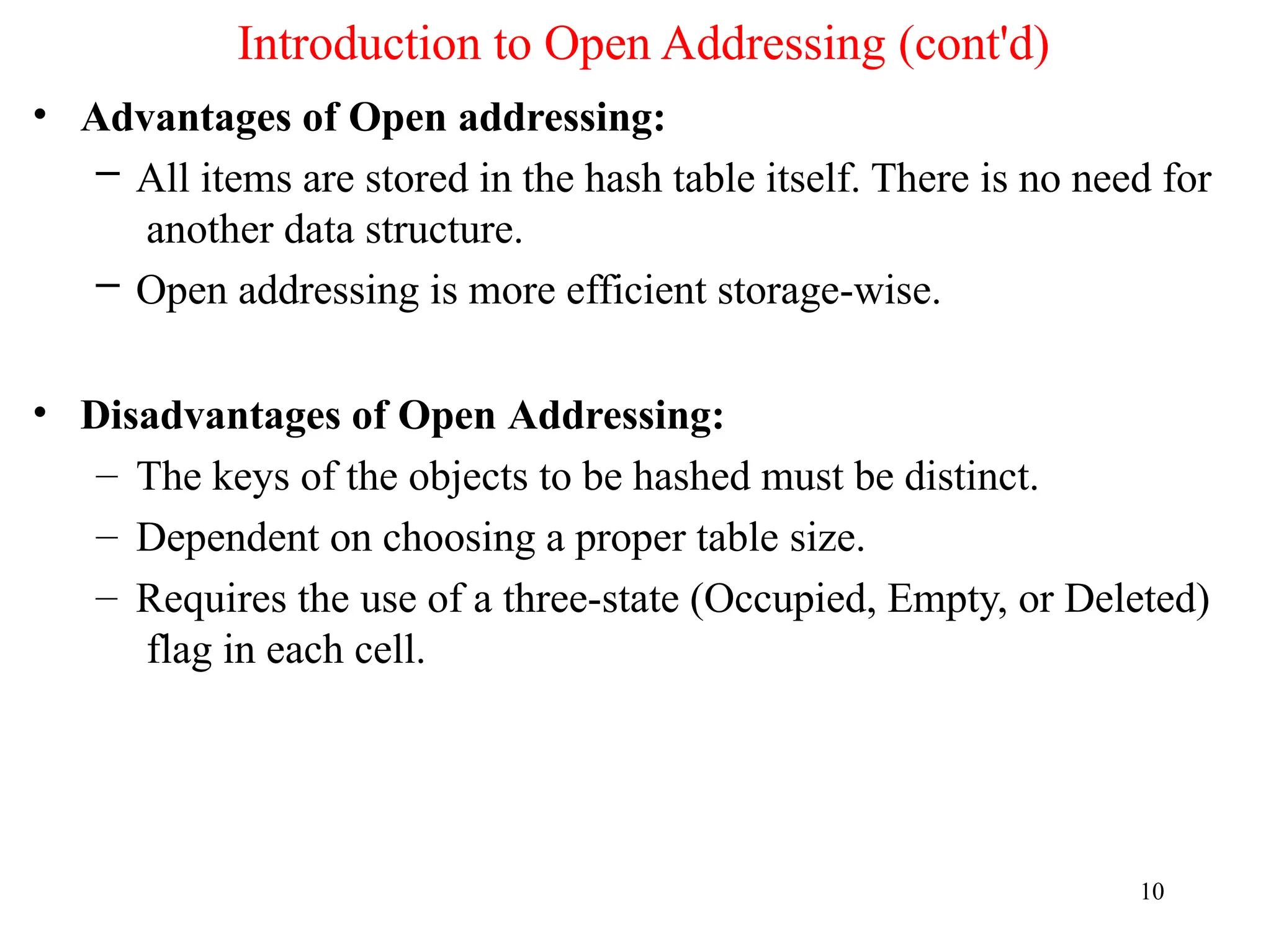
  Introduction to OpenAddressing (cont'd) 10 • Advantages of Open addressing: – All items are stored in the hash table itself. There is no need for another data structure. – Open addressing is more efficient storage-wise. • Disadvantages of Open Addressing: – The keys of the objects to be hashed must be distinct. – Dependent on choosing a proper table size. – Requires the use of a three-state (Occupied, Empty, or Deleted) flag in each cell.
• 11.
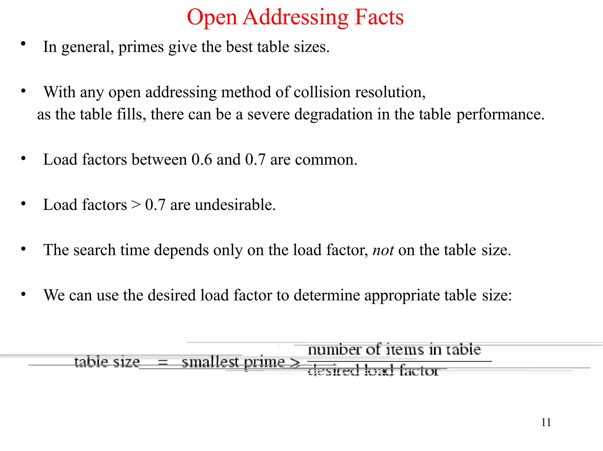
  Open Addressing Facts •In general, primes give the best table sizes. • With any open addressing method of collision resolution, as the table fills, there can be a severe degradation in the table performance. • Load factors between 0.6 and 0.7 are common. • Load factors > 0.7 are undesirable. • The search time depends only on the load factor, not on the table size. • We can use the desired load factor to determine appropriate table size: 11
• 12.
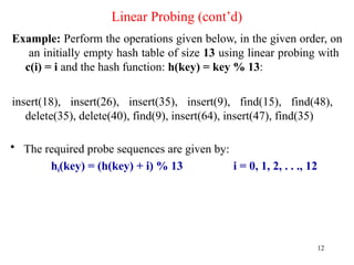
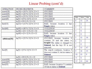
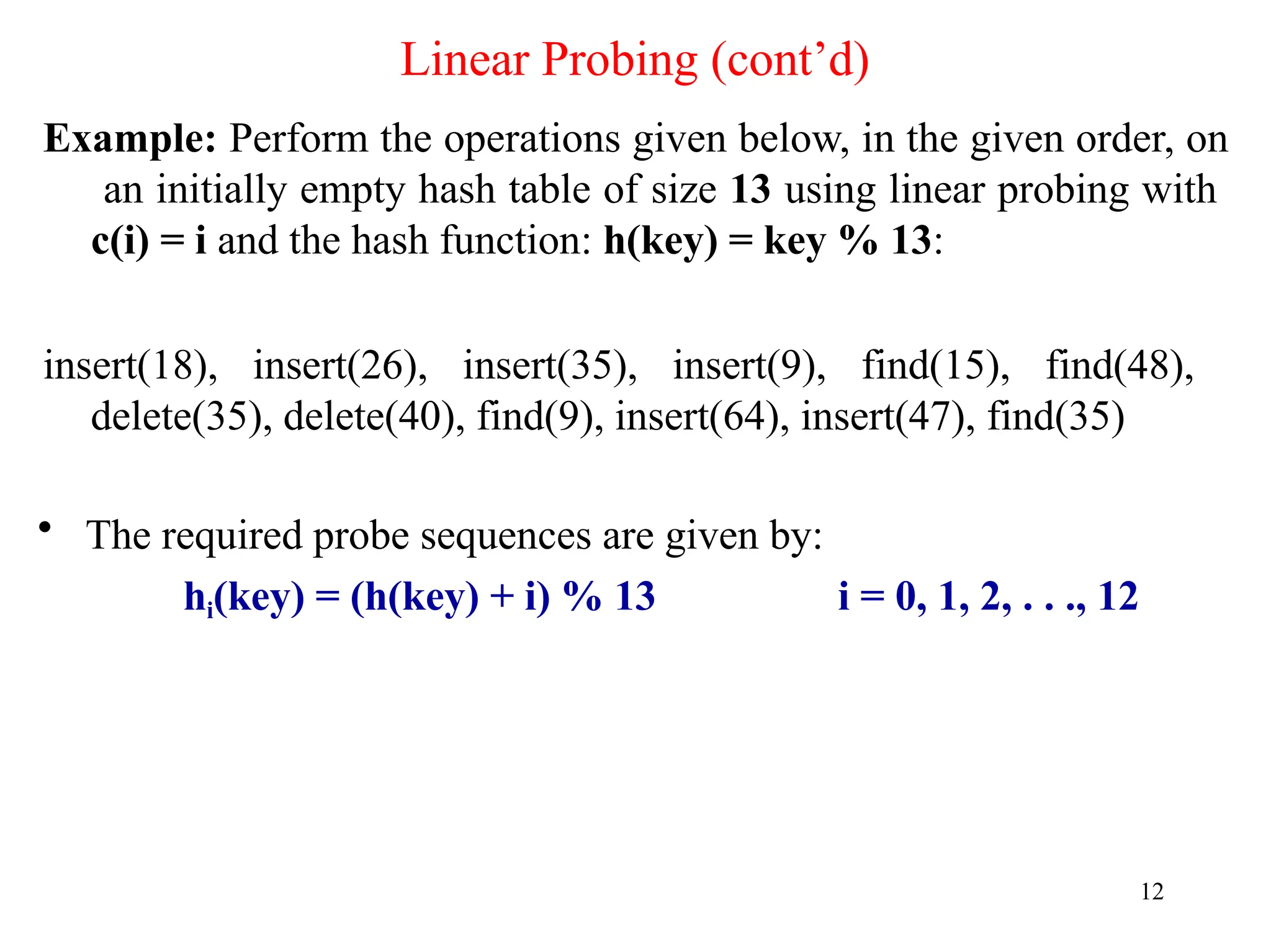
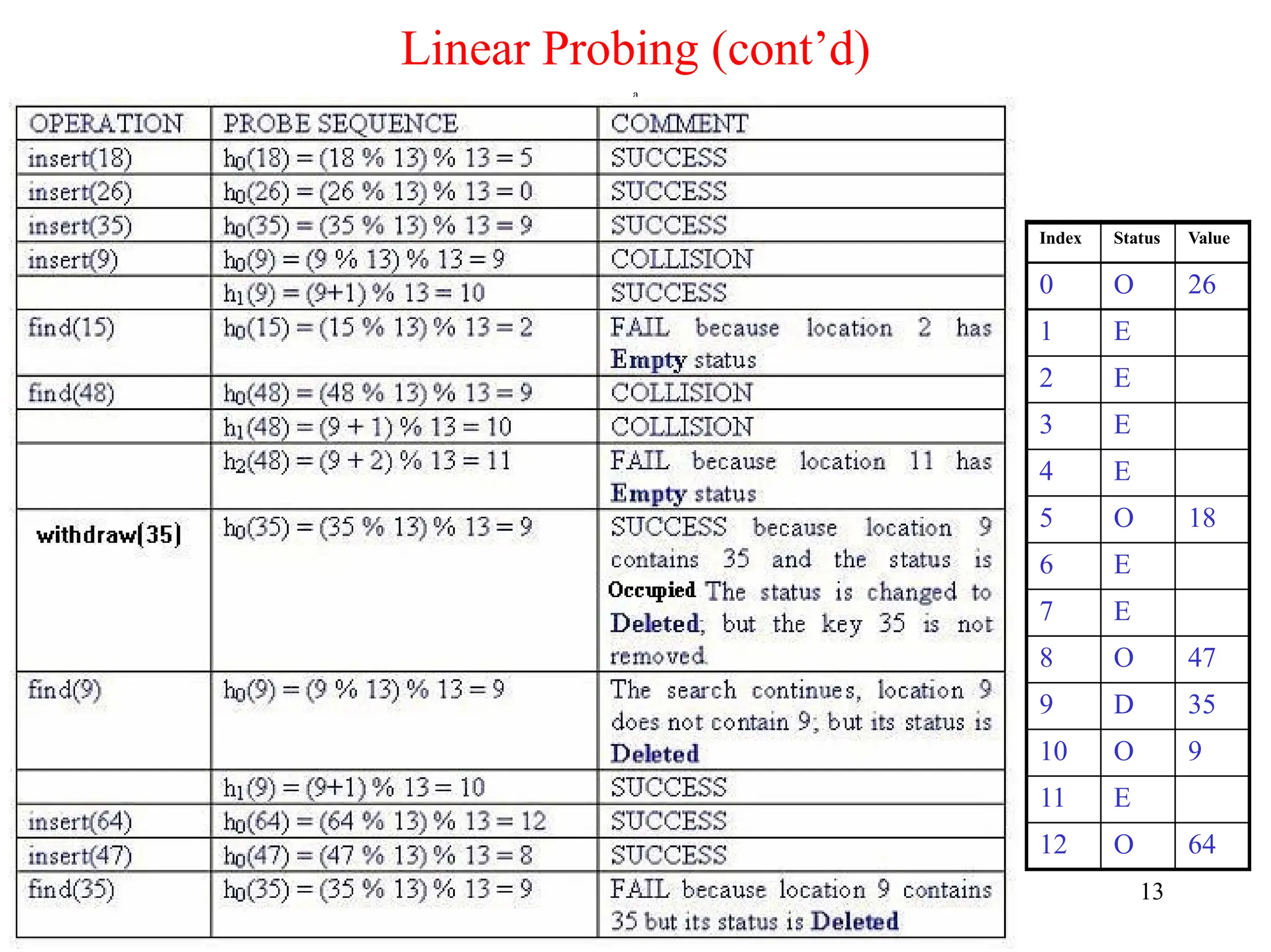
  Linear Probing (cont’d) 12 Example:Perform the operations given below, in the given order, on an initially empty hash table of size 13 using linear probing with c(i) = i and the hash function: h(key) = key % 13: insert(18), insert(26), insert(35), insert(9), find(15), find(48), delete(35), delete(40), find(9), insert(64), insert(47), find(35) • The required probe sequences are given by: hi(key) = (h(key) + i) % 13 i = 0, 1, 2, . . ., 12
• 13.
  Linear Probing (cont’d) a IndexStatus Value 0 O 26 1 E 2 E 3 E 4 E 5 O 18 6 E 7 E 8 O 47 9 D 35 10 O 9 11 E 12 O 64 13
• 14.
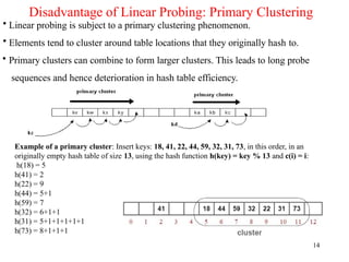
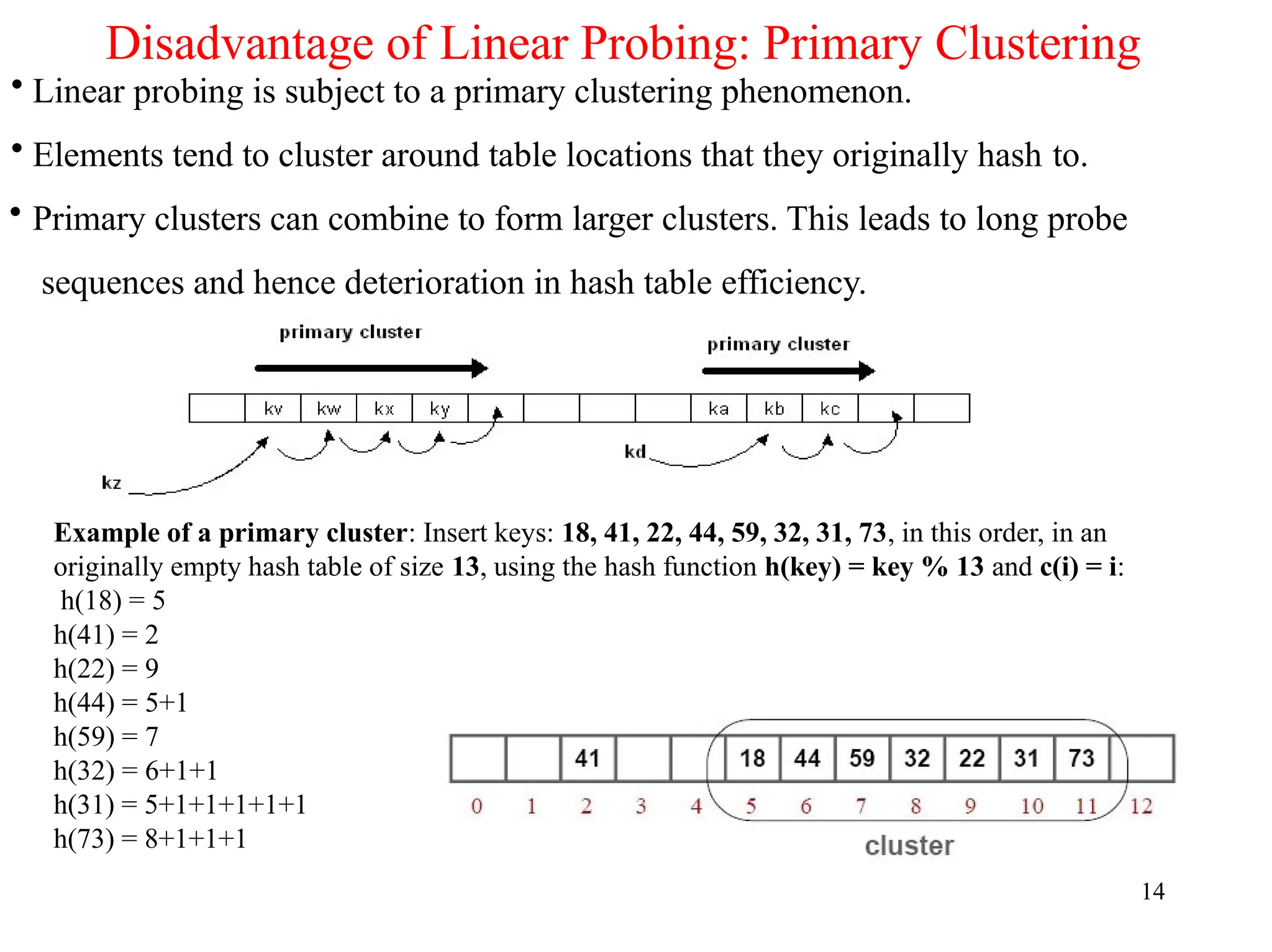
  Disadvantage of LinearProbing: Primary Clustering • Linear probing is subject to a primary clustering phenomenon. • Elements tend to cluster around table locations that they originally hash to. • Primary clusters can combine to form larger clusters. This leads to long probe sequences and hence deterioration in hash table efficiency. Example of a primary cluster: Insert keys: 18, 41, 22, 44, 59, 32, 31, 73, in this order, in an originally empty hash table of size 13, using the hash function h(key) = key % 13 and c(i) = i: h(18) = 5 h(41) = 2 h(22) = 9 h(44) = 5+1 h(59) = 7 h(32) = 6+1+1 h(31) = 5+1+1+1+1+1 h(73) = 8+1+1+1 14
• 15.
  Exercises 15 1. Given that, c(i)= a*i, for c(i) in linear probing, we discussed that this equation satisfies Property 2 only when a and n are relatively prime. Explain what the requirement of being relatively prime means in simple plain language. 2. Consider the general probe sequence, hi (r) = (h(r) + c(i))% n. Are we sure that if c(i) satisfies Property 2, then hi(r) will cover all n hash table locations, 0,1,...,n-1? Explain. 3. Suppose you are given k records to be loaded into a hash table of size n, with k < n using linear probing. Does the order in which these records are loaded matter for retrieval and insertion? Explain. 4. A prime number is always the best choice of a hash table size. Is this statement true or false? Justify your answer either way.