Downloaded 10 times


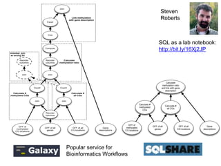
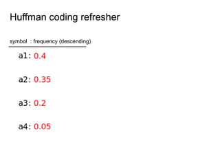
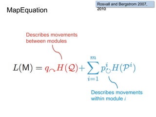
![“[This was hard] due to the large amount of data (e.g. data indexes for data retrieval,
dissection into data blocks and processing steps, order in which steps are performed
to match memory/time requirements, file formats required by software used).
In addition we actually spend quite some time in iterations fixing problems with
certain features (e.g. capping ENCODE data), testing features and feature products
to include, identifying useful test data sets, adjusting the training data (e.g. 1000G vs
human-derived variants)
So roughly 50% of the project was testing and improving the model, 30% figuring out
how to do things (engineering) and 20% getting files and getting them into the right
format.
I guess in total [I spent] 6 months [on this project].”
At least 3 months on issues of
scale, file handling, and feature
engineering.
Martin Kircher,
Genome SciencesWhy?
3k NSF postdocs in 2010
$50k / postdoc
at least 50% overhead
maybe $75M annually
at NSF alone?](https://image.slidesharecdn.com/mmds2014myriav2-140710163304-phpapp02/85/MMDS-2014-Myria-and-Scalable-Graph-Clustering-with-RelaxMap-7-320.jpg)


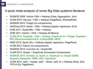
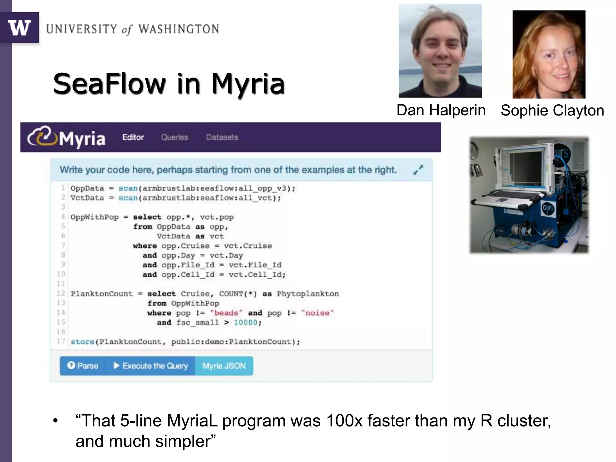
![SELECT x.strain, x.chr, x.region as snp_region, x.start_bp as snp_start_bp
, x.end_bp as snp_end_bp, w.start_bp as nc_start_bp, w.end_bp as nc_end_bp
, w.category as nc_category
, CASE WHEN (x.start_bp >= w.start_bp AND x.end_bp <= w.end_bp)
THEN x.end_bp - x.start_bp + 1
WHEN (x.start_bp <= w.start_bp AND w.start_bp <= x.end_bp)
THEN x.end_bp - w.start_bp + 1
WHEN (x.start_bp <= w.end_bp AND w.end_bp <= x.end_bp)
THEN w.end_bp - x.start_bp + 1
END AS len_overlap
FROM [koesterj@washington.edu].[hotspots_deserts.tab] x
INNER JOIN [koesterj@washington.edu].[table_noncoding_positions.tab] w
ON x.chr = w.chr
WHERE (x.start_bp >= w.start_bp AND x.end_bp <= w.end_bp)
OR (x.start_bp <= w.start_bp AND w.start_bp <= x.end_bp)
OR (x.start_bp <= w.end_bp AND w.end_bp <= x.end_bp)
ORDER BY x.strain, x.chr ASC, x.start_bp ASC
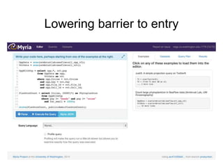
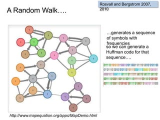
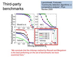
Non-programmers can write very complex queries
(rather than relying on staff programmers)
Example: Computing the overlaps of two sets of blast results
We see thousands of
queries written by
non-programmers](https://image.slidesharecdn.com/mmds2014myriav2-140710163304-phpapp02/85/MMDS-2014-Myria-and-Scalable-Graph-Clustering-with-RelaxMap-11-320.jpg)
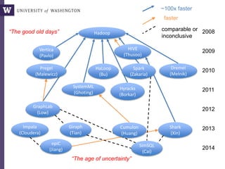
![14
A = LOAD('points.txt', id:int, x:float, y:float)
E = LIMIT(A, 4);
F = SEQUENCE();
Centroids = [FROM E EMIT (id=F.next, x=E.x, y=E.y)];
Kmeans = [FROM A EMIT (id=id, x=x, y=y, cluster_id=0)]
DO
I = CROSS(Kmeans, Centroids);
J = [FROM I EMIT (Kmeans.id, Kmeans.x, Kmeans.y, Centroids.cluster_id,
$distance(Kmeans.x, Kmeans.y, Centroids.x, Centroids.y))];
K = [FROM J EMIT id, distance=$min(distance)];
L = JOIN(J, id, K, id)
M = [FROM L WHERE J.distance <= K.distance EMIT
(id=J.id, x=J.x, y=J.y, cluster_id=J.cluster_id)];
Kmeans' = [FROM M EMIT (id, x, y, $min(cluster_id))];
Delta = DIFF(Kmeans', Kmeans)
Kmeans = Kmeans'
Centroids = [FROM Kmeans' EMIT (cluster_id, x=avg(x), y=avg(y))];
WHILE DELTA != {}
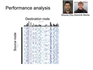
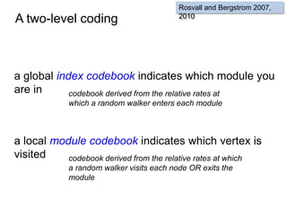
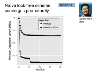
K-Means in relational algebra](https://image.slidesharecdn.com/mmds2014myriav2-140710163304-phpapp02/85/MMDS-2014-Myria-and-Scalable-Graph-Clustering-with-RelaxMap-14-320.jpg)


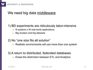


![32
A = LOAD('points.txt', id:int, x:float, y:float)
E = LIMIT(A, 4);
F = SEQUENCE();
Centroids = [FROM E EMIT (id=F.next, x=E.x, y=E.y)];
Kmeans = [FROM A EMIT (id=id, x=x, y=y, cluster_id=0)]
DO
I = CROSS(Kmeans, Centroids);
J = [FROM I EMIT (Kmeans.id, Kmeans.x, Kmeans.y, Centroids.cluster_id,
$distance(Kmeans.x, Kmeans.y, Centroids.x, Centroids.y))];
K = [FROM J EMIT id, distance=$min(distance)];
L = JOIN(J, id, K, id)
M = [FROM L WHERE J.distance <= K.distance EMIT
(id=J.id, x=J.x, y=J.y, cluster_id=J.cluster_id)];
Kmeans' = [FROM M EMIT (id, x, y, $min(cluster_id))];
Delta = DIFF(Kmeans', Kmeans)
Kmeans = Kmeans'
Centroids = [FROM Kmeans' EMIT (cluster_id, x=avg(x), y=avg(y))];
WHILE DELTA != {}
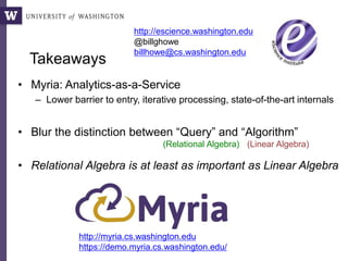
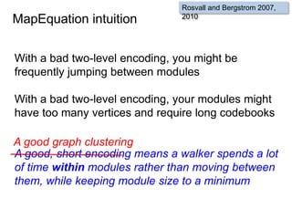
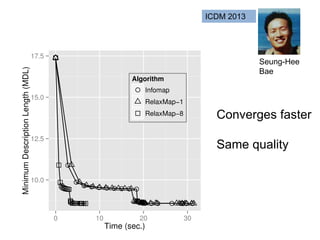
K-Means in the language MyriaL](https://image.slidesharecdn.com/mmds2014myriav2-140710163304-phpapp02/85/MMDS-2014-Myria-and-Scalable-Graph-Clustering-with-RelaxMap-32-320.jpg)
![33
CurGood = SCAN(public:adhoc:sc_points);
DO
mean = [FROM CurGood EMIT val=AVG(v)];
std = [FROM CurGood EMIT val=STDEV(v)];
NewBad = [FROM Good WHERE ABS(Good.v - mean) > 2 * std EMIT *];
CurGood = CurGood - NewBad;
continue = [FROM NewBad EMIT COUNT(NewBad.v) > 0];
WHILE continue;
DUMP(CurGood);
Sigma-clipping, V0
Sigma-Clipping (v1)](https://image.slidesharecdn.com/mmds2014myriav2-140710163304-phpapp02/85/MMDS-2014-Myria-and-Scalable-Graph-Clustering-with-RelaxMap-33-320.jpg)
![34
CurGood = P
sum = [FROM CurGood EMIT SUM(val)];
sumsq = [FROM CurGood EMIT SUM(val*val)]
cnt = [FROM CurGood EMIT CNT(*)];
NewBad = []
DO
sum = sum – [FROM NewBad EMIT SUM(val)];
sumsq = sum – [FROM NewBad EMIT SUM(val*val)];
cnt = sum - [FROM NewBad EMIT CNT(*)];
mean = sum / cnt
std = sqrt(1/(cnt*(cnt-1)) * (cnt * sumsq - sum*sum))
NewBad = FILTER([ABS(val-mean)>std], CurGood)
CurGood = CurGood - NewBad
WHILE NewBad != {}
Sigma-clipping, V1: Incremental
Sigma-Clipping (v2)](https://image.slidesharecdn.com/mmds2014myriav2-140710163304-phpapp02/85/MMDS-2014-Myria-and-Scalable-Graph-Clustering-with-RelaxMap-34-320.jpg)
![35
Points = SCAN(public:adhoc:sc_points);
aggs = [FROM Points EMIT _sum=SUM(v), sumsq=SUM(v*v), cnt=COUNT(v)];
newBad = []
bounds = [FROM Points EMIT lower=MIN(v), upper=MAX(v)];
DO
new_aggs = [FROM newBad EMIT _sum=SUM(v), sumsq=SUM(v*v), cnt=COUNT(v)];
aggs = [FROM aggs, new_aggs EMIT _sum=aggs._sum - new_aggs._sum,
sumsq=aggs.sumsq - new_aggs.sumsq, cnt=aggs.cnt - new_aggs.cnt];
stats = [FROM aggs EMIT mean=_sum/cnt,
std=SQRT(1.0/(cnt*(cnt-1)) * (cnt * sumsq - _sum * _sum))];
newBounds = [FROM stats EMIT lower=mean - 2 * std, upper=mean + 2 * std];
tooLow = [FROM Points, bounds, newBounds WHERE newBounds.lower > v
AND v >= bounds.lower EMIT v=Points.v];
tooHigh = [FROM Points, bounds, newBounds WHERE newBounds.upper < v
AND v <= bounds.upper EMIT v=Points.v];
newBad = UNIONALL(tooLow, tooHigh);
bounds = newBounds;
continue = [FROM newBad EMIT COUNT(v) > 0];
WHILE continue;
output = [FROM Points, bounds WHERE Points.v > bounds.lower AND
Points.v < bounds.upper EMIT v=Points.v];
DUMP(output);
Sigma-clipping, V2
Sigma-Clipping (v3)](https://image.slidesharecdn.com/mmds2014myriav2-140710163304-phpapp02/85/MMDS-2014-Myria-and-Scalable-Graph-Clustering-with-RelaxMap-35-320.jpg)


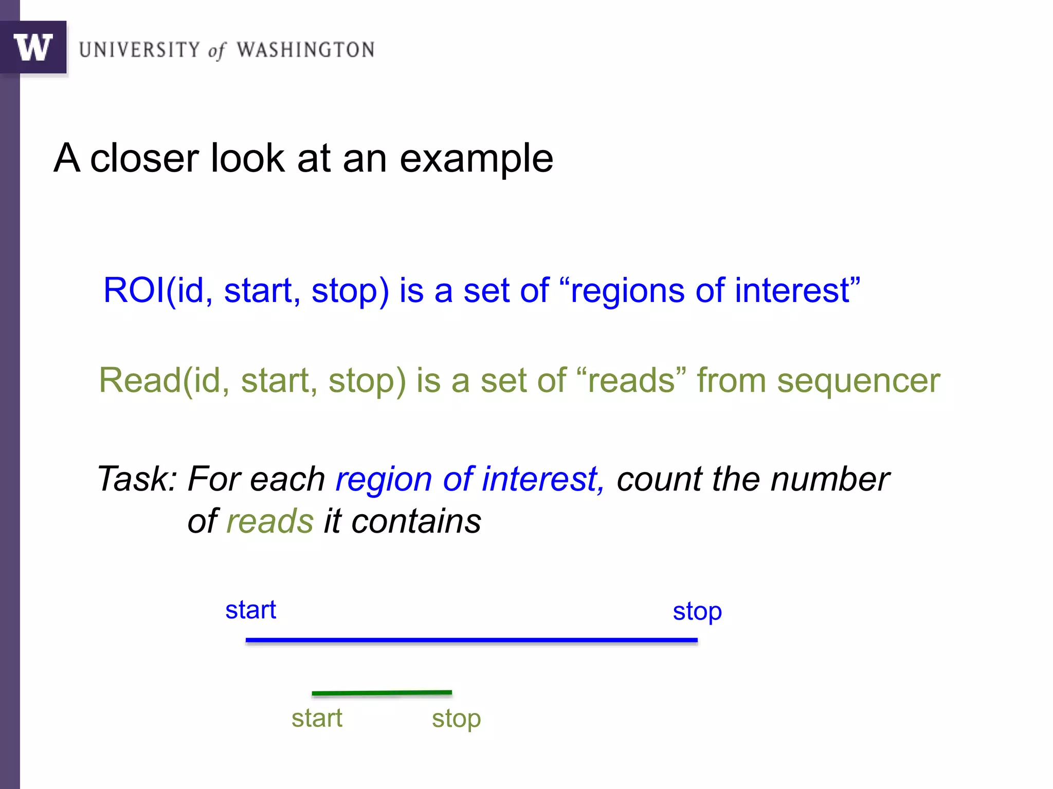
![SELECT roi.id, count(rd.id)
FROM regions_of_interest roi, reads rd
WHERE roi.start <= rd.start AND rd.[end] <= roi.[end]
GROUP BY roi.id
As a query
“region of interest”
sequence “read”](https://image.slidesharecdn.com/mmds2014myriav2-140710163304-phpapp02/85/MMDS-2014-Myria-and-Scalable-Graph-Clustering-with-RelaxMap-58-320.jpg)
![SELECT roi.id, count(rd.start)
FROM regions_of_interest roi, reads rd
WHERE roi.start <= rd.start AND rd.[end] <= roi.[end]
GROUP BY roi.id
Why databases get
a bad reputation
many minutes
SELECT roi.id, count(rd.start) as cnt
FROM regions_of_interest roi, indexed_reads rd
WHERE roi.start <= rd.start AND rd.start <= roi.[end]
AND roi.start <= rd.[end] AND rd.[end] >= roi.[end]
GROUP BY roi.id
3 seconds!
roi
read
two-sided index scan
one-sided index scan,
plus filter
The broken promise of declarative query…](https://image.slidesharecdn.com/mmds2014myriav2-140710163304-phpapp02/85/MMDS-2014-Myria-and-Scalable-Graph-Clustering-with-RelaxMap-59-320.jpg)


![“[This was hard] due to the large amount of data (e.g. data indexes for data retrieval,
dissection into data blocks and processing steps, order in which steps are performed
to match memory/time requirements, file formats required by software used).
In addition we actually spend quite some time in iterations fixing problems with
certain features (e.g. capping ENCODE data), testing features and feature products
to include, identifying useful test data sets, adjusting the training data (e.g. 1000G vs
human-derived variants)
So roughly 50% of the project was testing and improving the model, 30% figuring out
how to do things (engineering) and 20% getting files and getting them into the right
format.
I guess in total [I spent] 6 months [on this project].”
At least 3 months on issues of
scale, file handling, and feature
engineering.
Martin Kircher,
Genome SciencesWhy?
3k NSF postdocs in 2010
$50k / postdoc
at least 50% overhead
maybe $75M annually
at NSF alone?](https://image.slidesharecdn.com/mmds2014myriav2-140710163304-phpapp02/75/MMDS-2014-Myria-and-Scalable-Graph-Clustering-with-RelaxMap-7-2048.jpg)
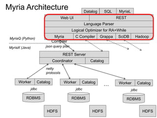
![SELECT x.strain, x.chr, x.region as snp_region, x.start_bp as snp_start_bp
, x.end_bp as snp_end_bp, w.start_bp as nc_start_bp, w.end_bp as nc_end_bp
, w.category as nc_category
, CASE WHEN (x.start_bp >= w.start_bp AND x.end_bp <= w.end_bp)
THEN x.end_bp - x.start_bp + 1
WHEN (x.start_bp <= w.start_bp AND w.start_bp <= x.end_bp)
THEN x.end_bp - w.start_bp + 1
WHEN (x.start_bp <= w.end_bp AND w.end_bp <= x.end_bp)
THEN w.end_bp - x.start_bp + 1
END AS len_overlap
FROM [koesterj@washington.edu].[hotspots_deserts.tab] x
INNER JOIN [koesterj@washington.edu].[table_noncoding_positions.tab] w
ON x.chr = w.chr
WHERE (x.start_bp >= w.start_bp AND x.end_bp <= w.end_bp)
OR (x.start_bp <= w.start_bp AND w.start_bp <= x.end_bp)
OR (x.start_bp <= w.end_bp AND w.end_bp <= x.end_bp)
ORDER BY x.strain, x.chr ASC, x.start_bp ASC
Non-programmers can write very complex queries
(rather than relying on staff programmers)
Example: Computing the overlaps of two sets of blast results
We see thousands of
queries written by
non-programmers](https://image.slidesharecdn.com/mmds2014myriav2-140710163304-phpapp02/75/MMDS-2014-Myria-and-Scalable-Graph-Clustering-with-RelaxMap-11-2048.jpg)


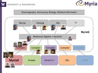
![14
A = LOAD('points.txt', id:int, x:float, y:float)
E = LIMIT(A, 4);
F = SEQUENCE();
Centroids = [FROM E EMIT (id=F.next, x=E.x, y=E.y)];
Kmeans = [FROM A EMIT (id=id, x=x, y=y, cluster_id=0)]
DO
I = CROSS(Kmeans, Centroids);
J = [FROM I EMIT (Kmeans.id, Kmeans.x, Kmeans.y, Centroids.cluster_id,
$distance(Kmeans.x, Kmeans.y, Centroids.x, Centroids.y))];
K = [FROM J EMIT id, distance=$min(distance)];
L = JOIN(J, id, K, id)
M = [FROM L WHERE J.distance <= K.distance EMIT
(id=J.id, x=J.x, y=J.y, cluster_id=J.cluster_id)];
Kmeans' = [FROM M EMIT (id, x, y, $min(cluster_id))];
Delta = DIFF(Kmeans', Kmeans)
Kmeans = Kmeans'
Centroids = [FROM Kmeans' EMIT (cluster_id, x=avg(x), y=avg(y))];
WHILE DELTA != {}
K-Means in relational algebra](https://image.slidesharecdn.com/mmds2014myriav2-140710163304-phpapp02/75/MMDS-2014-Myria-and-Scalable-Graph-Clustering-with-RelaxMap-14-2048.jpg)


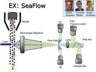
![32
A = LOAD('points.txt', id:int, x:float, y:float)
E = LIMIT(A, 4);
F = SEQUENCE();
Centroids = [FROM E EMIT (id=F.next, x=E.x, y=E.y)];
Kmeans = [FROM A EMIT (id=id, x=x, y=y, cluster_id=0)]
DO
I = CROSS(Kmeans, Centroids);
J = [FROM I EMIT (Kmeans.id, Kmeans.x, Kmeans.y, Centroids.cluster_id,
$distance(Kmeans.x, Kmeans.y, Centroids.x, Centroids.y))];
K = [FROM J EMIT id, distance=$min(distance)];
L = JOIN(J, id, K, id)
M = [FROM L WHERE J.distance <= K.distance EMIT
(id=J.id, x=J.x, y=J.y, cluster_id=J.cluster_id)];
Kmeans' = [FROM M EMIT (id, x, y, $min(cluster_id))];
Delta = DIFF(Kmeans', Kmeans)
Kmeans = Kmeans'
Centroids = [FROM Kmeans' EMIT (cluster_id, x=avg(x), y=avg(y))];
WHILE DELTA != {}
K-Means in the language MyriaL](https://image.slidesharecdn.com/mmds2014myriav2-140710163304-phpapp02/75/MMDS-2014-Myria-and-Scalable-Graph-Clustering-with-RelaxMap-32-2048.jpg)
![33
CurGood = SCAN(public:adhoc:sc_points);
DO
mean = [FROM CurGood EMIT val=AVG(v)];
std = [FROM CurGood EMIT val=STDEV(v)];
NewBad = [FROM Good WHERE ABS(Good.v - mean) > 2 * std EMIT *];
CurGood = CurGood - NewBad;
continue = [FROM NewBad EMIT COUNT(NewBad.v) > 0];
WHILE continue;
DUMP(CurGood);
Sigma-clipping, V0
Sigma-Clipping (v1)](https://image.slidesharecdn.com/mmds2014myriav2-140710163304-phpapp02/75/MMDS-2014-Myria-and-Scalable-Graph-Clustering-with-RelaxMap-33-2048.jpg)
![34
CurGood = P
sum = [FROM CurGood EMIT SUM(val)];
sumsq = [FROM CurGood EMIT SUM(val*val)]
cnt = [FROM CurGood EMIT CNT(*)];
NewBad = []
DO
sum = sum – [FROM NewBad EMIT SUM(val)];
sumsq = sum – [FROM NewBad EMIT SUM(val*val)];
cnt = sum - [FROM NewBad EMIT CNT(*)];
mean = sum / cnt
std = sqrt(1/(cnt*(cnt-1)) * (cnt * sumsq - sum*sum))
NewBad = FILTER([ABS(val-mean)>std], CurGood)
CurGood = CurGood - NewBad
WHILE NewBad != {}
Sigma-clipping, V1: Incremental
Sigma-Clipping (v2)](https://image.slidesharecdn.com/mmds2014myriav2-140710163304-phpapp02/75/MMDS-2014-Myria-and-Scalable-Graph-Clustering-with-RelaxMap-34-2048.jpg)
![35
Points = SCAN(public:adhoc:sc_points);
aggs = [FROM Points EMIT _sum=SUM(v), sumsq=SUM(v*v), cnt=COUNT(v)];
newBad = []
bounds = [FROM Points EMIT lower=MIN(v), upper=MAX(v)];
DO
new_aggs = [FROM newBad EMIT _sum=SUM(v), sumsq=SUM(v*v), cnt=COUNT(v)];
aggs = [FROM aggs, new_aggs EMIT _sum=aggs._sum - new_aggs._sum,
sumsq=aggs.sumsq - new_aggs.sumsq, cnt=aggs.cnt - new_aggs.cnt];
stats = [FROM aggs EMIT mean=_sum/cnt,
std=SQRT(1.0/(cnt*(cnt-1)) * (cnt * sumsq - _sum * _sum))];
newBounds = [FROM stats EMIT lower=mean - 2 * std, upper=mean + 2 * std];
tooLow = [FROM Points, bounds, newBounds WHERE newBounds.lower > v
AND v >= bounds.lower EMIT v=Points.v];
tooHigh = [FROM Points, bounds, newBounds WHERE newBounds.upper < v
AND v <= bounds.upper EMIT v=Points.v];
newBad = UNIONALL(tooLow, tooHigh);
bounds = newBounds;
continue = [FROM newBad EMIT COUNT(v) > 0];
WHILE continue;
output = [FROM Points, bounds WHERE Points.v > bounds.lower AND
Points.v < bounds.upper EMIT v=Points.v];
DUMP(output);
Sigma-clipping, V2
Sigma-Clipping (v3)](https://image.slidesharecdn.com/mmds2014myriav2-140710163304-phpapp02/75/MMDS-2014-Myria-and-Scalable-Graph-Clustering-with-RelaxMap-35-2048.jpg)


![SELECT roi.id, count(rd.id)
FROM regions_of_interest roi, reads rd
WHERE roi.start <= rd.start AND rd.[end] <= roi.[end]
GROUP BY roi.id
As a query
“region of interest”
sequence “read”](https://image.slidesharecdn.com/mmds2014myriav2-140710163304-phpapp02/75/MMDS-2014-Myria-and-Scalable-Graph-Clustering-with-RelaxMap-58-2048.jpg)
![SELECT roi.id, count(rd.start)
FROM regions_of_interest roi, reads rd
WHERE roi.start <= rd.start AND rd.[end] <= roi.[end]
GROUP BY roi.id
Why databases get
a bad reputation
many minutes
SELECT roi.id, count(rd.start) as cnt
FROM regions_of_interest roi, indexed_reads rd
WHERE roi.start <= rd.start AND rd.start <= roi.[end]
AND roi.start <= rd.[end] AND rd.[end] >= roi.[end]
GROUP BY roi.id
3 seconds!
roi
read
two-sided index scan
one-sided index scan,
plus filter
The broken promise of declarative query…](https://image.slidesharecdn.com/mmds2014myriav2-140710163304-phpapp02/75/MMDS-2014-Myria-and-Scalable-Graph-Clustering-with-RelaxMap-59-2048.jpg)


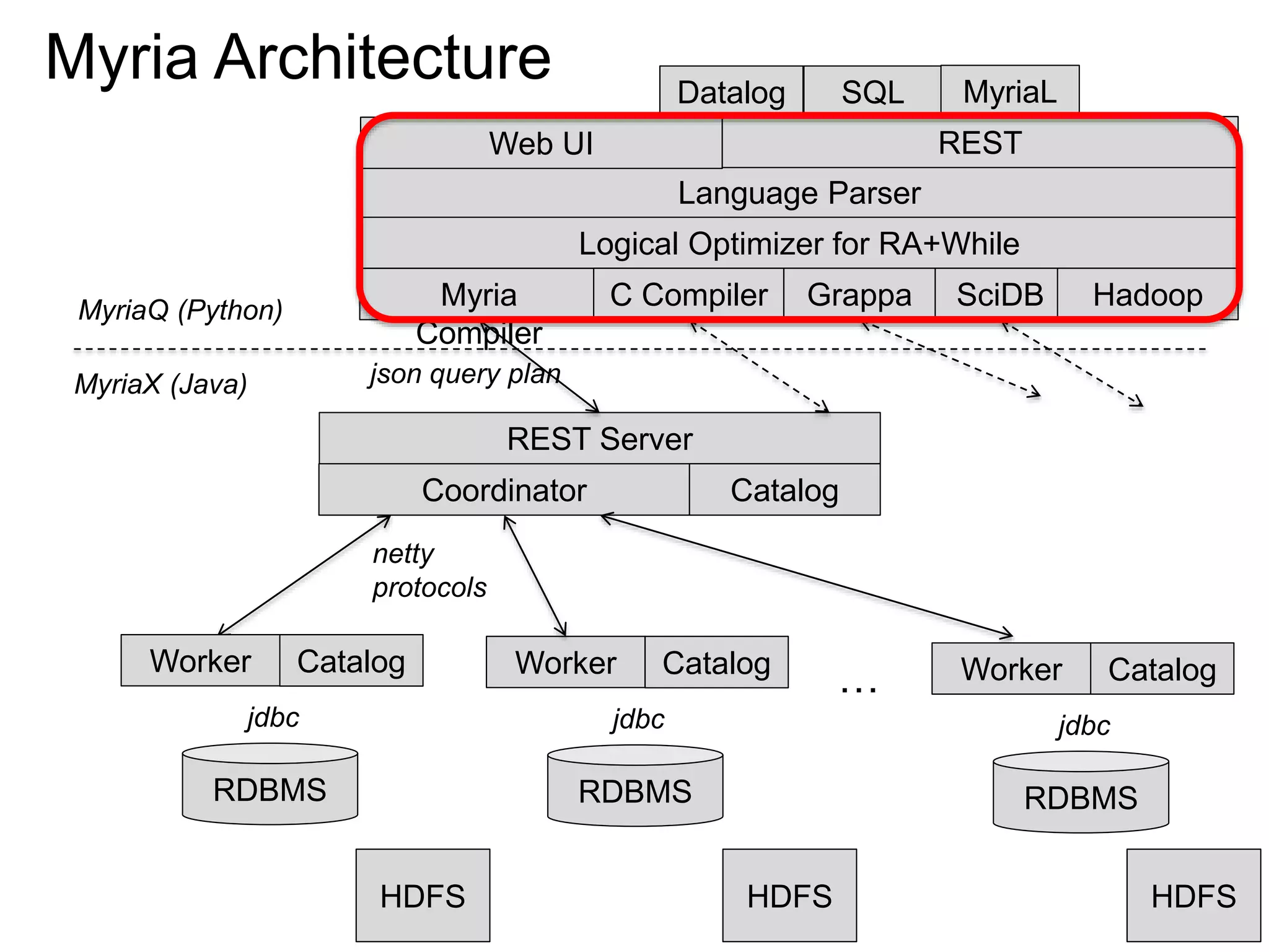
The document discusses Myria, a scalable analytics-as-a-service platform developed by researchers from the University of Washington, aimed at improving big data workflows and reducing the time spent on data handling. It highlights three key observations about big data challenges, including the inefficiency of current systems, the labor-intensive nature of big data experiments, and the need for distributed, federated databases. Furthermore, it emphasizes Myria's architecture and features, such as its optimizing compiler and iterative execution engine, which enable faster and easier data analytics.


