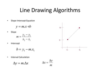
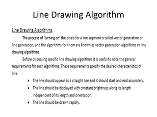
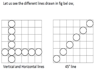
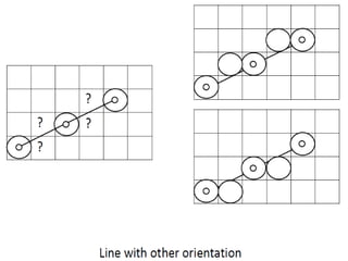
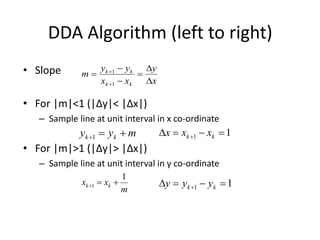
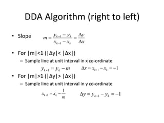
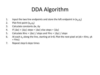
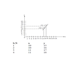
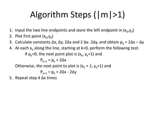
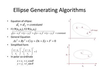
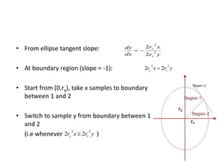
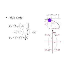
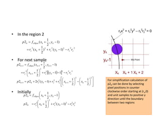
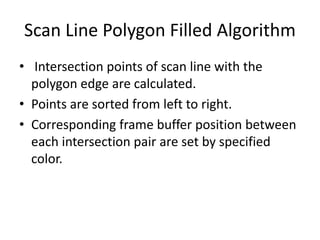
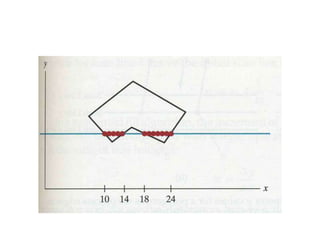
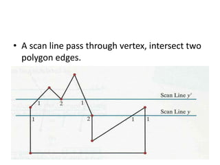
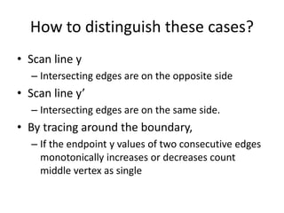
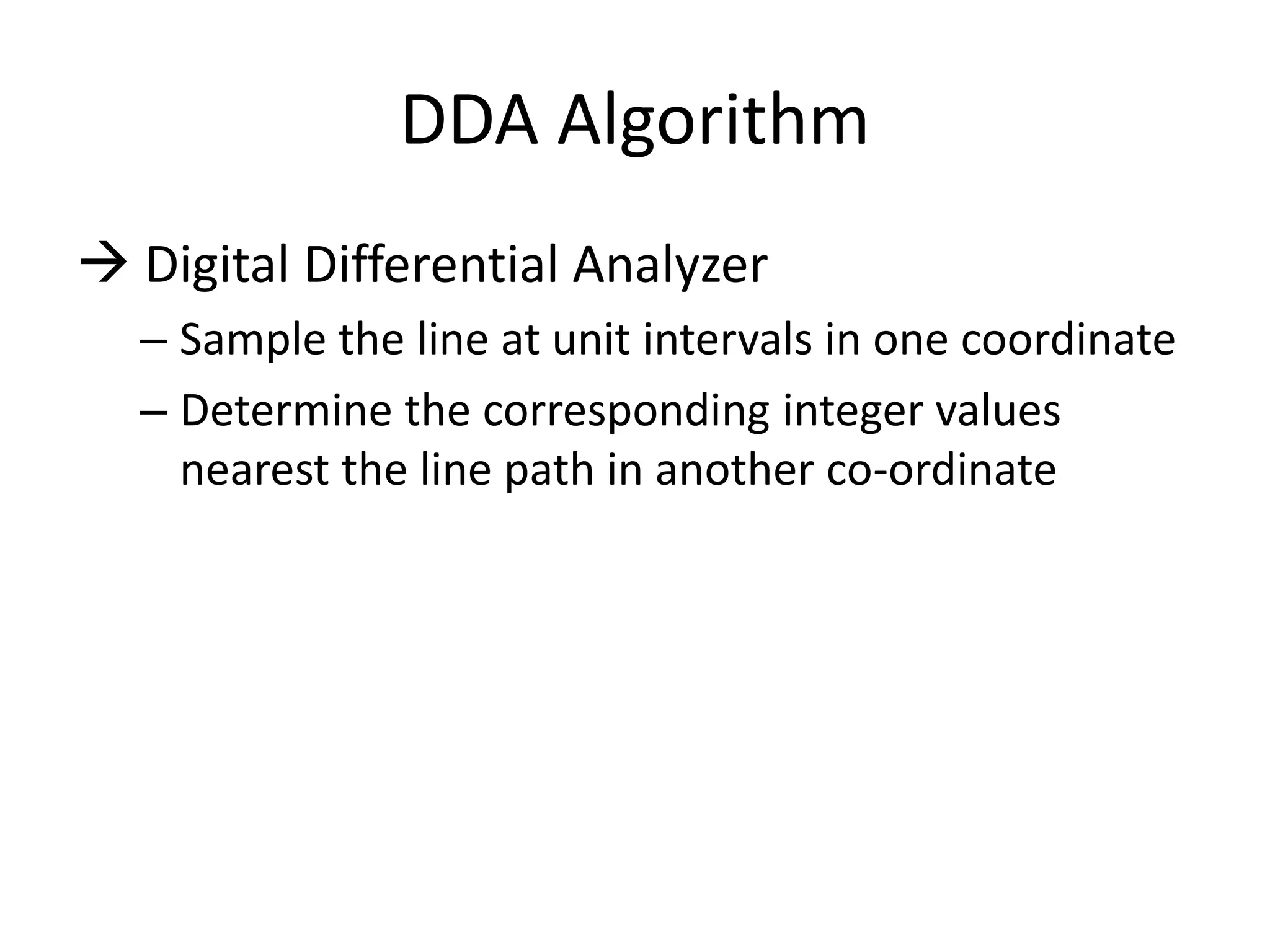
The document covers various algorithms for rendering geometric shapes in computer graphics, including line drawing algorithms like DDA and Bresenham’s, as well as circle and ellipse generating algorithms. It explains the fundamental concepts of points, lines, and the computational principles behind these algorithms, detailing their steps and pseudo code for implementation. Additionally, it highlights the importance of using integer calculations for efficiency in pixel plotting.


![Defining decision parameter
[1]
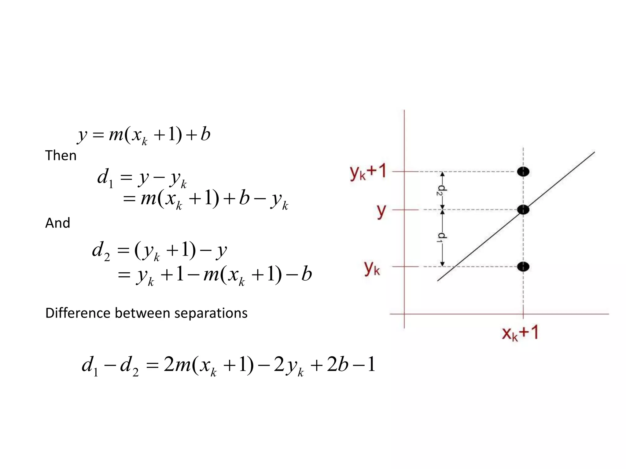
Sign of pk is same as that of d1-d2 for Δx>0 (left to right sampling)
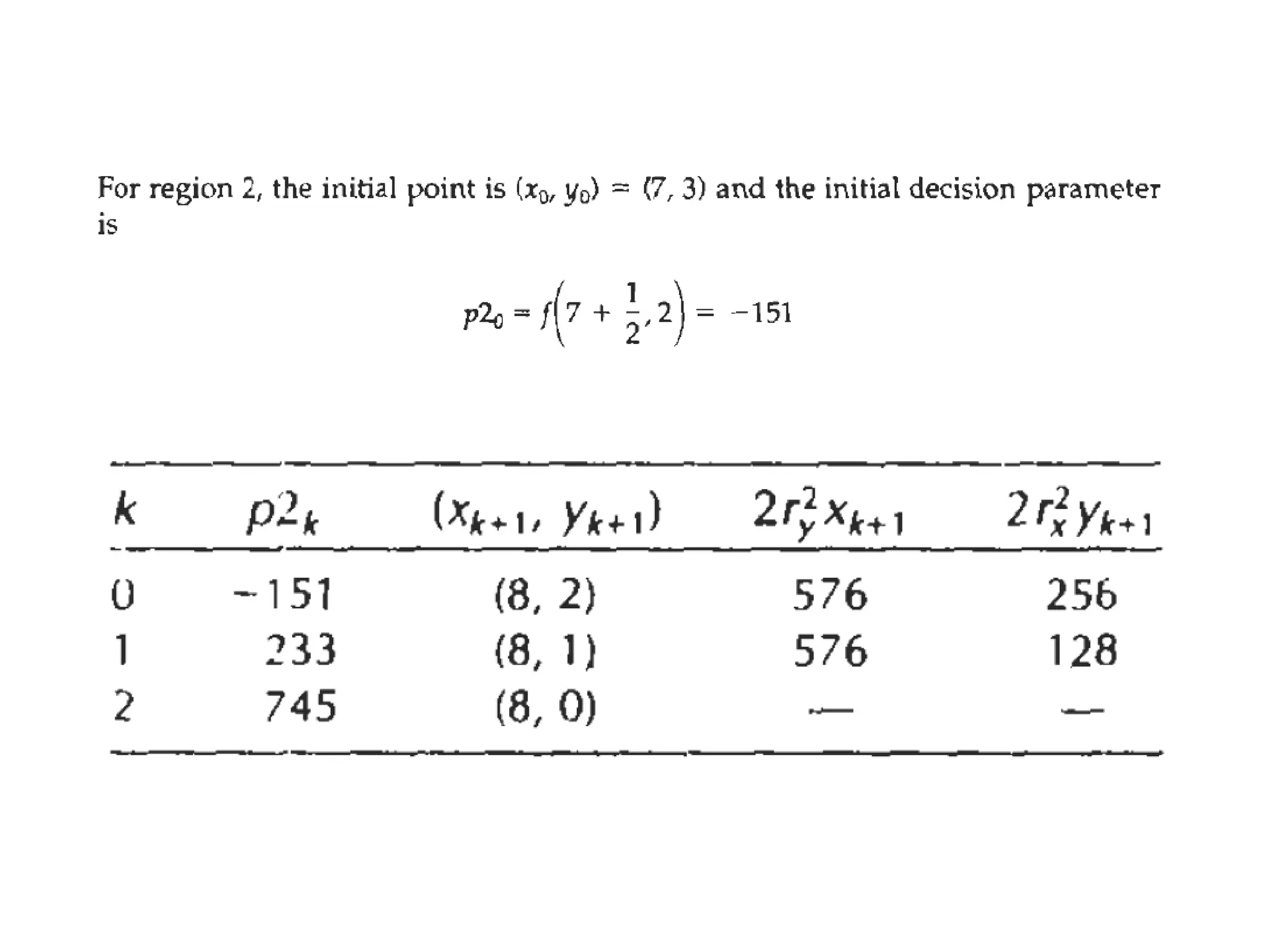
For Recursive calculation, initially
cyxxy kk .2.2
Constant=2Δy + Δx(2b-1) Which is
independent of pixel position
cyxxyp kkk 111 .2.2
)(2)(2 111 kkkkkk yyxxxypp
c eliminated here
)(22 11 kkkk yyxypp
because xk+1 = xk + 1
yk+1-yk = 0 if pk < 0
yk+1-yk = 1 if pk ≥ 0
xyp 20
Substitute b = y0 – m.x0
and m = Δy/Δx in [1]
)( 21 ddxpk ](https://image.slidesharecdn.com/4-150810041938-lva1-app6892/85/Output-primitives-in-Computer-Graphics-21-320.jpg)


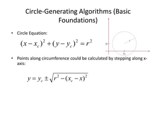


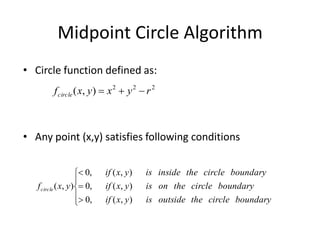
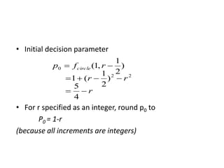
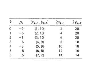
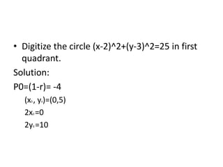
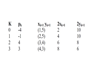
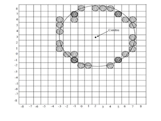
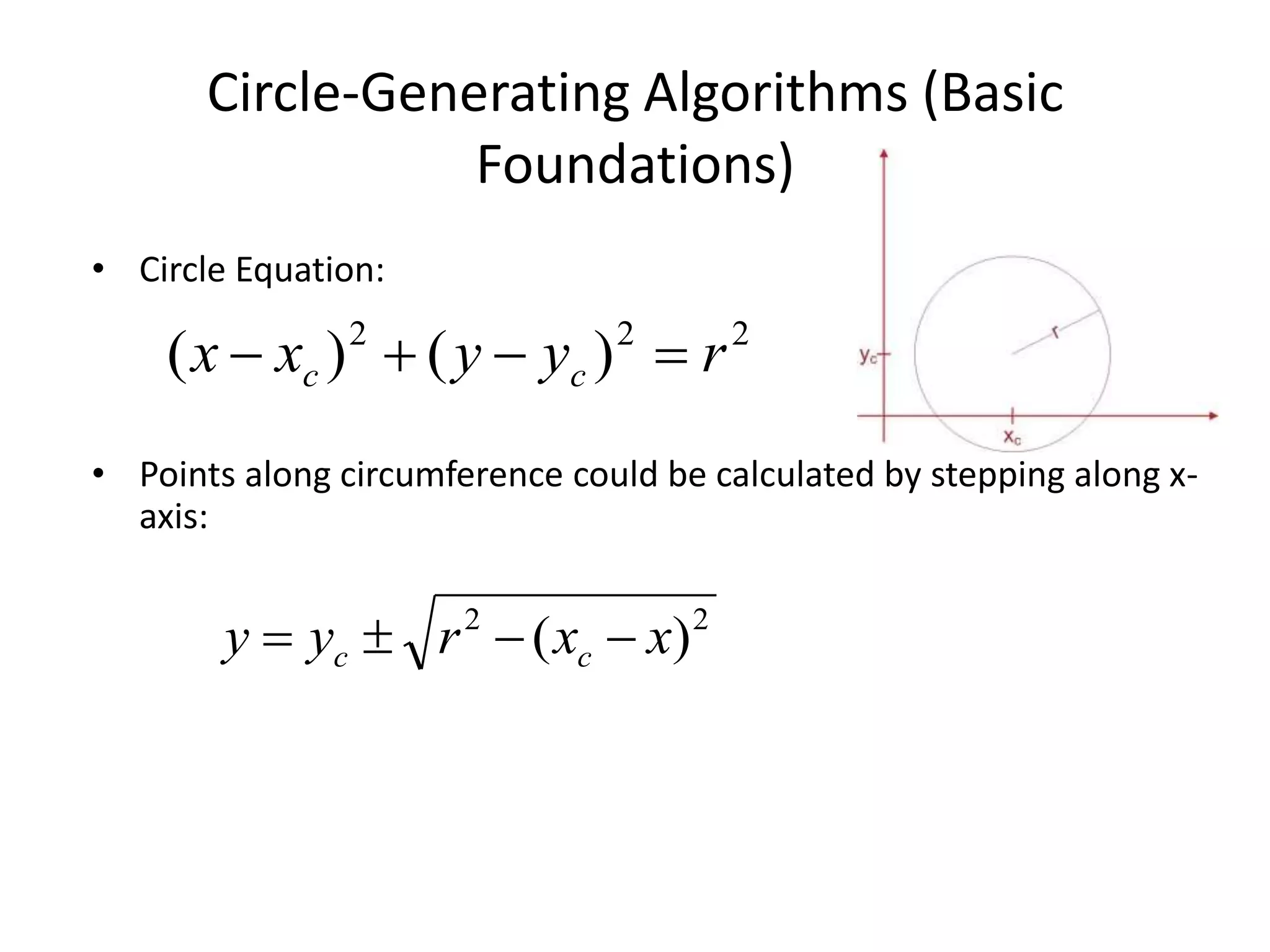
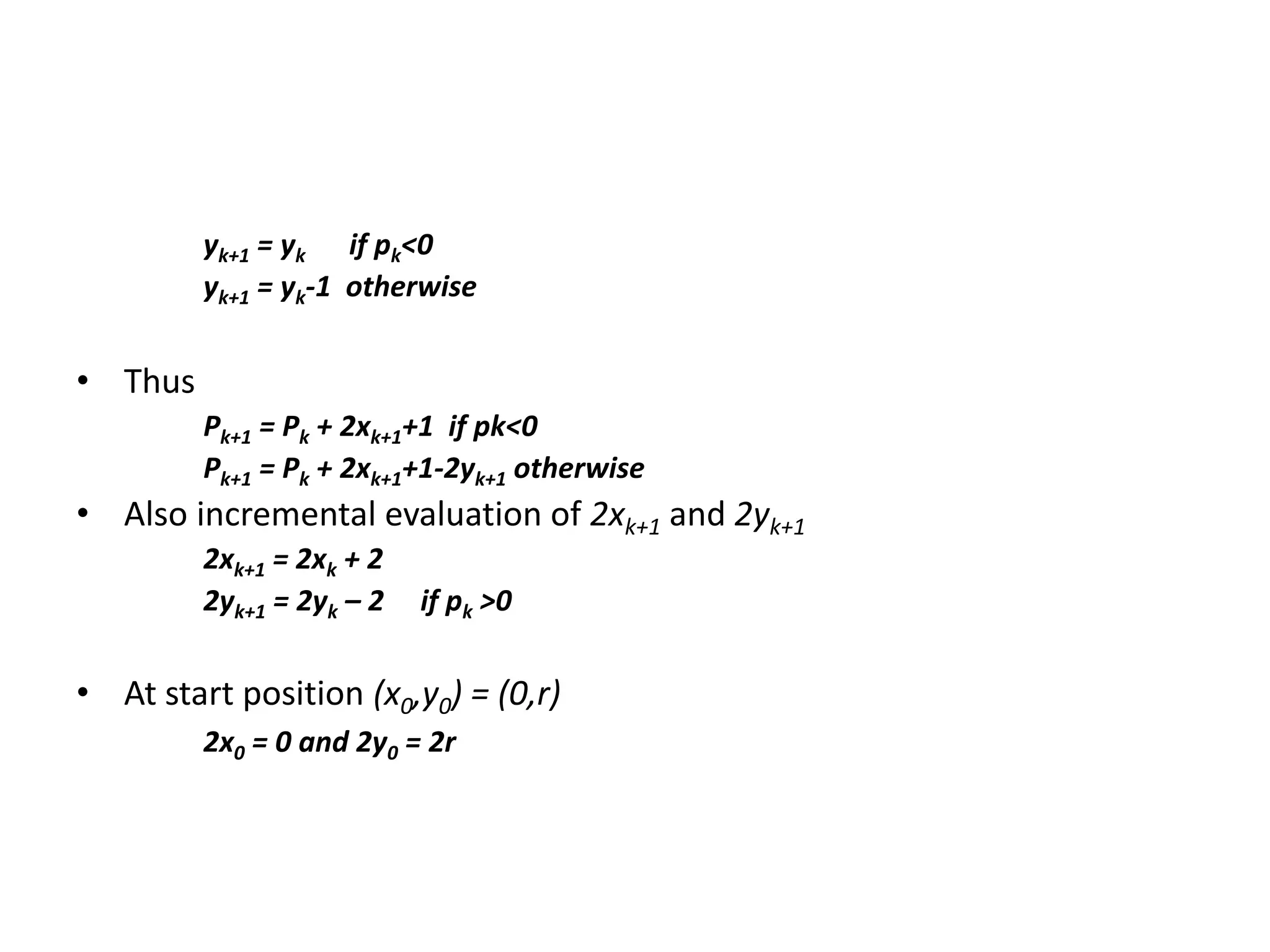
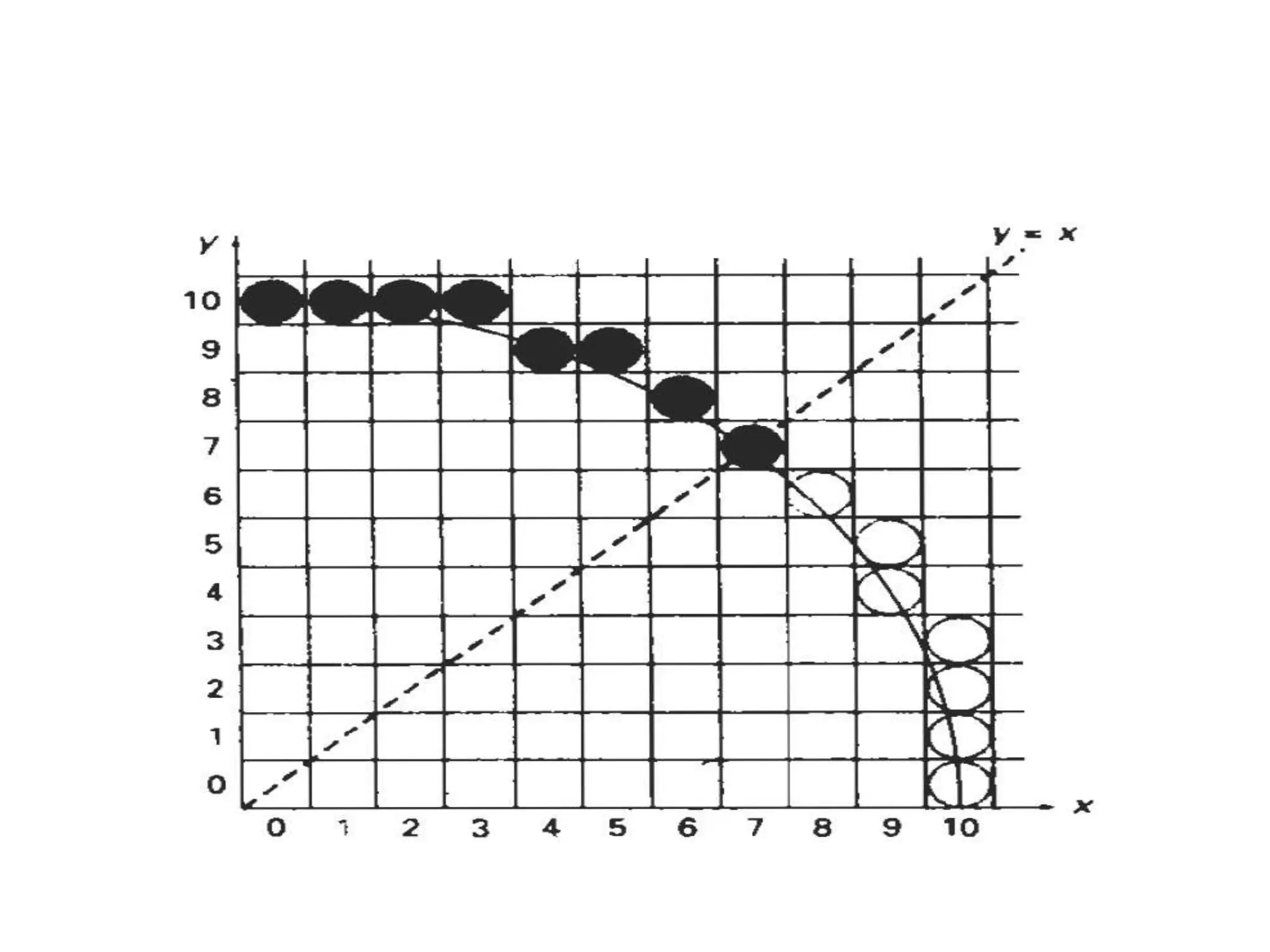
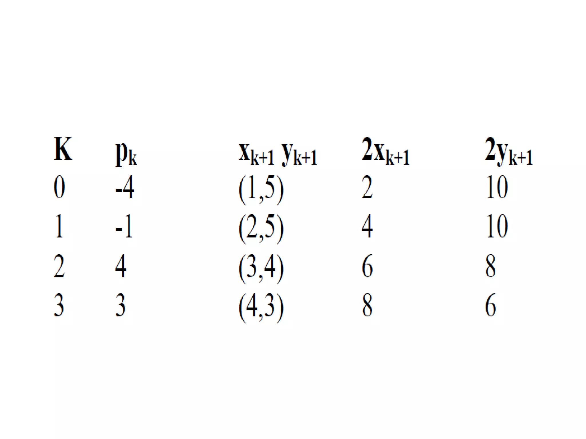
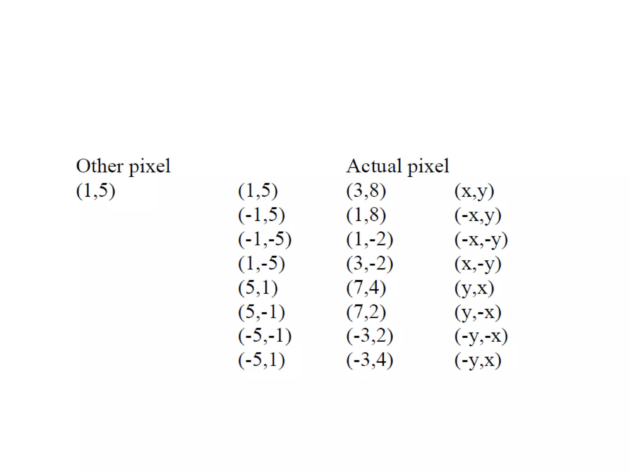
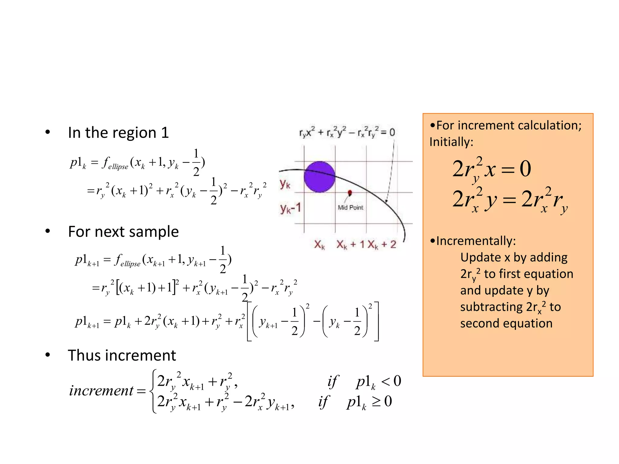
![• Decision parameter is the circle function; evaluated as:
222
)
2
1
()1(
)
2
1
,1(
ryx
yxfp
kk
kkcirclek
1)()()1(2
)
2
1
(]1)1[(
)
2
1
,1(
1
22
11
22
1
2
111
kkkkkkk
kk
kkcirclek
yyyyxpp
ryx
yxfp](https://image.slidesharecdn.com/4-150810041938-lva1-app6892/85/Output-primitives-in-Computer-Graphics-39-320.jpg)


![Defining decision parameter
[1]
Sign of pk is same as that of d1-d2 for Δx>0 (left to right sampling)
For Recursive calculation, initially
cyxxy kk .2.2
Constant=2Δy + Δx(2b-1) Which is
independent of pixel position
cyxxyp kkk 111 .2.2
)(2)(2 111 kkkkkk yyxxxypp
c eliminated here
)(22 11 kkkk yyxypp
because xk+1 = xk + 1
yk+1-yk = 0 if pk < 0
yk+1-yk = 1 if pk ≥ 0
xyp 20
Substitute b = y0 – m.x0
and m = Δy/Δx in [1]
)( 21 ddxpk ](https://image.slidesharecdn.com/4-150810041938-lva1-app6892/75/Output-primitives-in-Computer-Graphics-21-2048.jpg)


![• Decision parameter is the circle function; evaluated as:
222
)
2
1
()1(
)
2
1
,1(
ryx
yxfp
kk
kkcirclek
1)()()1(2
)
2
1
(]1)1[(
)
2
1
,1(
1
22
11
22
1
2
111
kkkkkkk
kk
kkcirclek
yyyyxpp
ryx
yxfp](https://image.slidesharecdn.com/4-150810041938-lva1-app6892/75/Output-primitives-in-Computer-Graphics-39-2048.jpg)


![Chapter 3 - Part 1 [Autosaved].pptx](https://cdn.slidesharecdn.com/ss_thumbnails/chapter3-part1autosaved-230109040832-9344385c-thumbnail.jpg?width=600ounds&width=560&fit=bounds)


