Downloaded 122 times


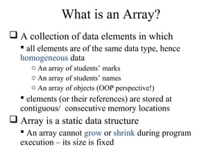


![Using Arrays
Array_name[index]
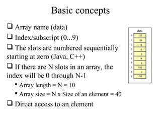
For example, in Java
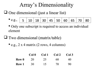
System.out.println(data[4]) will display
0
data[3] = 99 will replace -3 with 99](https://image.slidesharecdn.com/part3arraysandsearchingalgorithms-140828232254-phpapp02/85/Data-Structures-Part3-arrays-and-searching-algorithms-8-320.jpg)
![Some more concepts
data[ -1 ] always illegal
data[ 10 ] illegal (10 > upper bound)
data[ 1.5 ] always illegal
data[ 0 ] always OK
data[ 9 ] OK
Q. What will be the output of?
1.data[5] + 10
2.data[3] = data[3] + 10](https://image.slidesharecdn.com/part3arraysandsearchingalgorithms-140828232254-phpapp02/85/Data-Structures-Part3-arrays-and-searching-algorithms-9-320.jpg)
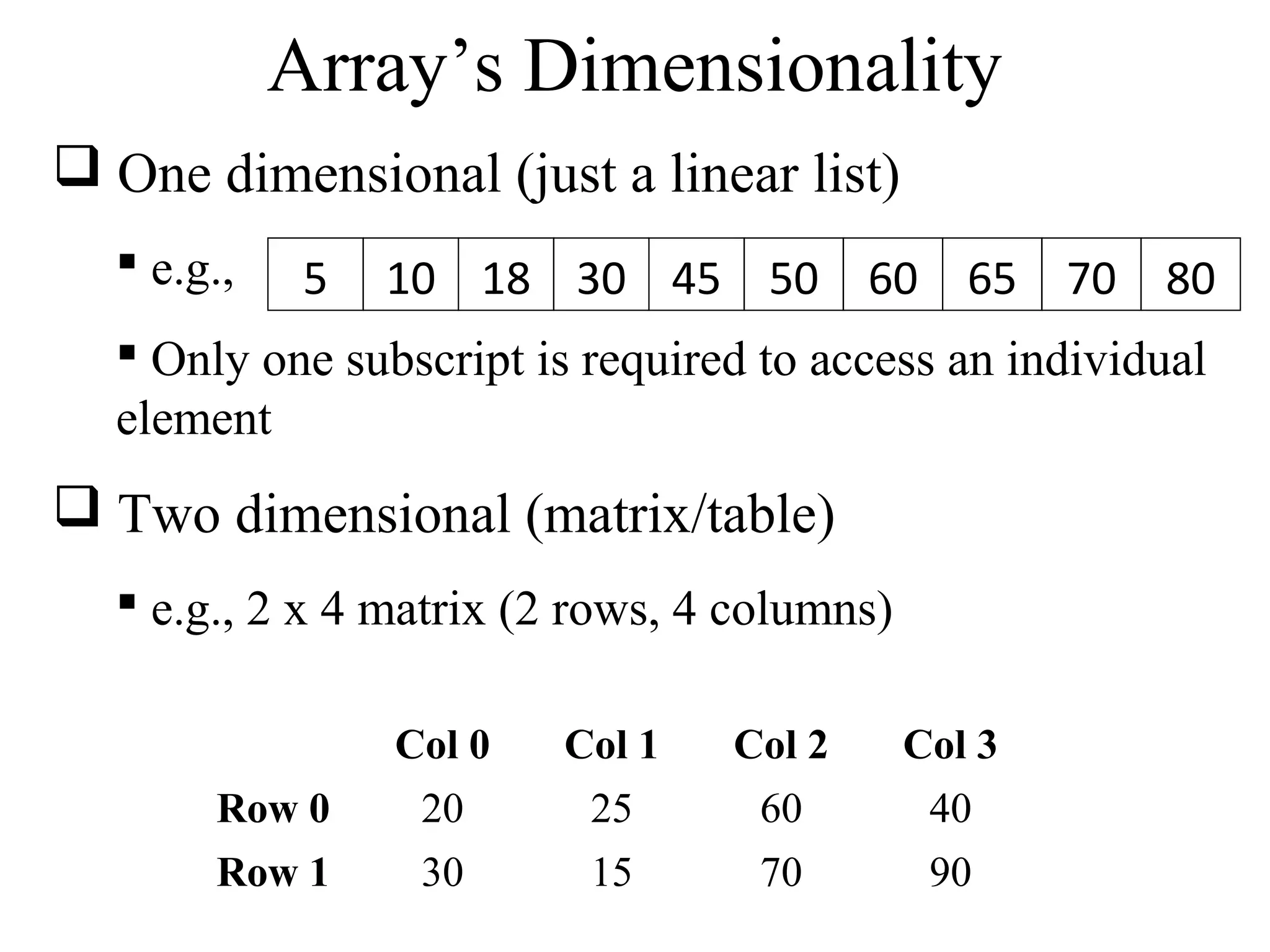
![Two dimensional Arrays
Let, the name of the two dimensional array is M
20 25 60 40
30 15 70 90
Two indices/subscripts are required (row,
column)
First element is at row 0, column 0
M0,0 or M(0, 0) or M[0][0] (more common)
What is: M[1][2]? M[3][4]?](https://image.slidesharecdn.com/part3arraysandsearchingalgorithms-140828232254-phpapp02/85/Data-Structures-Part3-arrays-and-searching-algorithms-11-320.jpg)
![Array Operations
Indexing: inspect or update an element using its index.
Performance is very fast O(1)
randomNumber = numbers[5];
numbers[20000] = 100;
Insertion: add an element at certain index
– Start: very slow O(n) because of shift
– End : very fast O(1) because no need to shift
Removal: remove an element at certain index
– Start: very slow O(n) because of shift
– End : very fast O(1) because no need to shift
Search: performance depends on algorithm
1) Linear: slow O(n) 2) binary : O(log n)
Sort: performance depends on algorithm
1) Bubble: slow O(n2) 2) Selection: slow O(n2)
3) Insertion: slow O(n2) 4)Merge : O (n log n)](https://image.slidesharecdn.com/part3arraysandsearchingalgorithms-140828232254-phpapp02/85/Data-Structures-Part3-arrays-and-searching-algorithms-12-320.jpg)
![One Dimensional Arrays in Java
To declare an array follow the type with (empty) []s
int[] grade; //or
int grade[]; //both declare an int array
In Java arrays are objects so must be created with the new
keyword
To create an array of ten integers:
int[] grade = new int[10];
Note that the array size has to be specified, although it can be
specified with a variable at run-time](https://image.slidesharecdn.com/part3arraysandsearchingalgorithms-140828232254-phpapp02/85/Data-Structures-Part3-arrays-and-searching-algorithms-13-320.jpg)
![Arrays in Java
When the array is created memory is reserved for its contents
Initialization lists can be used to specify the initial values of an
array, in which case the new operator is not used
int[] grade = {87, 93, 35}; //array of 3 ints
To find the length of an array use its .length property
int numGrades = grade.length; //note: not .length()!!](https://image.slidesharecdn.com/part3arraysandsearchingalgorithms-140828232254-phpapp02/85/Data-Structures-Part3-arrays-and-searching-algorithms-14-320.jpg)


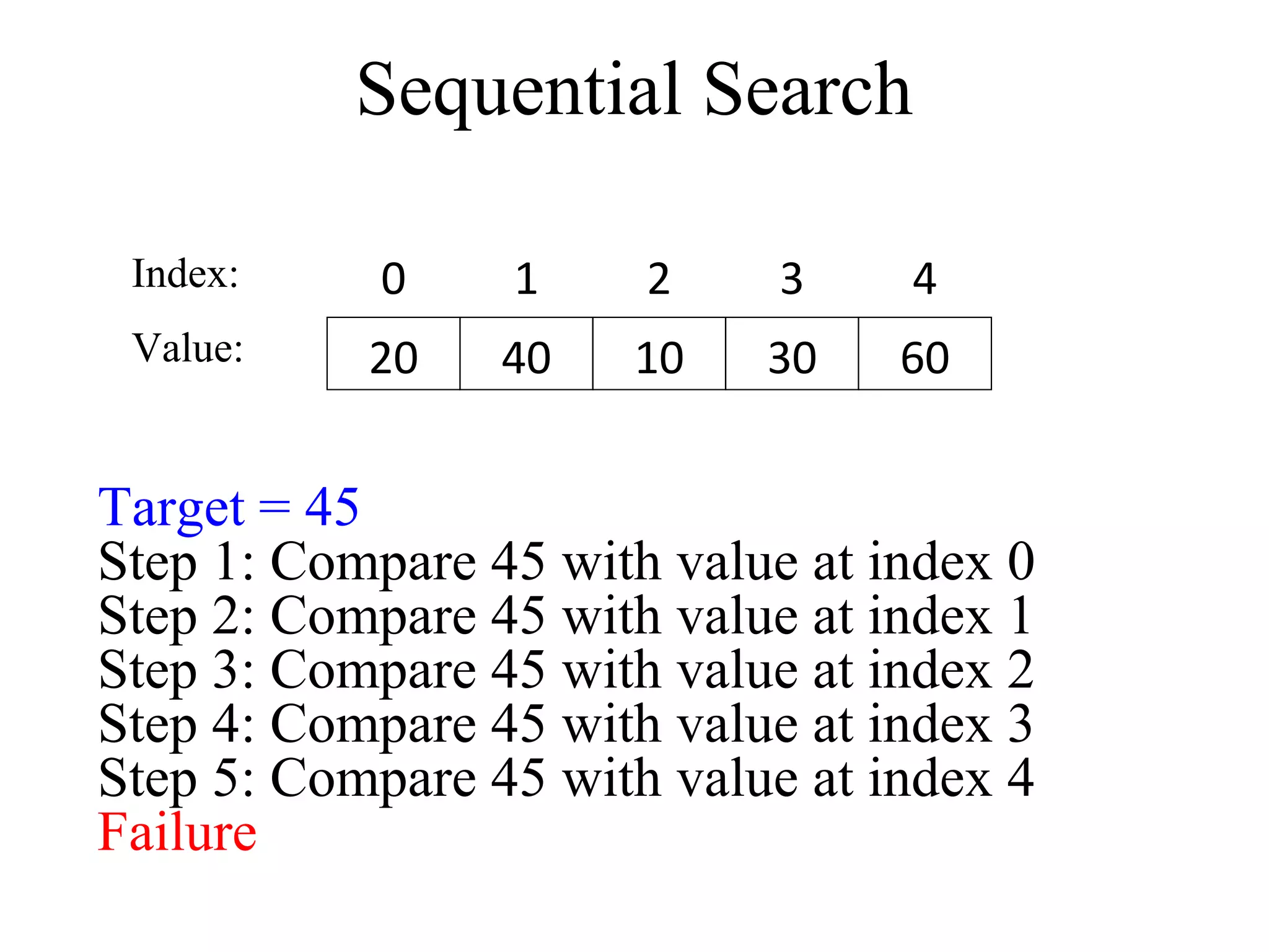
![Sequential Search Algorithm
Given: A list of N elements, and the target
1. index 0
2. Repeat steps 3 to 5
3. Compare target with list[index]
4. if target = list[index] then
return index // success
else if index >= N - 1
return -1 // failure
5. index index + 1](https://image.slidesharecdn.com/part3arraysandsearchingalgorithms-140828232254-phpapp02/85/Data-Structures-Part3-arrays-and-searching-algorithms-20-320.jpg)

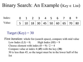

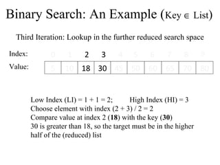


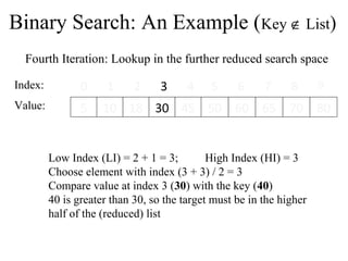
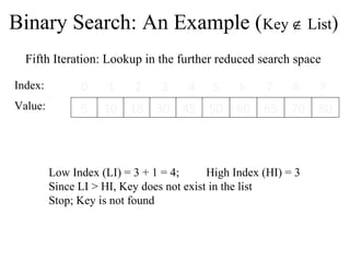
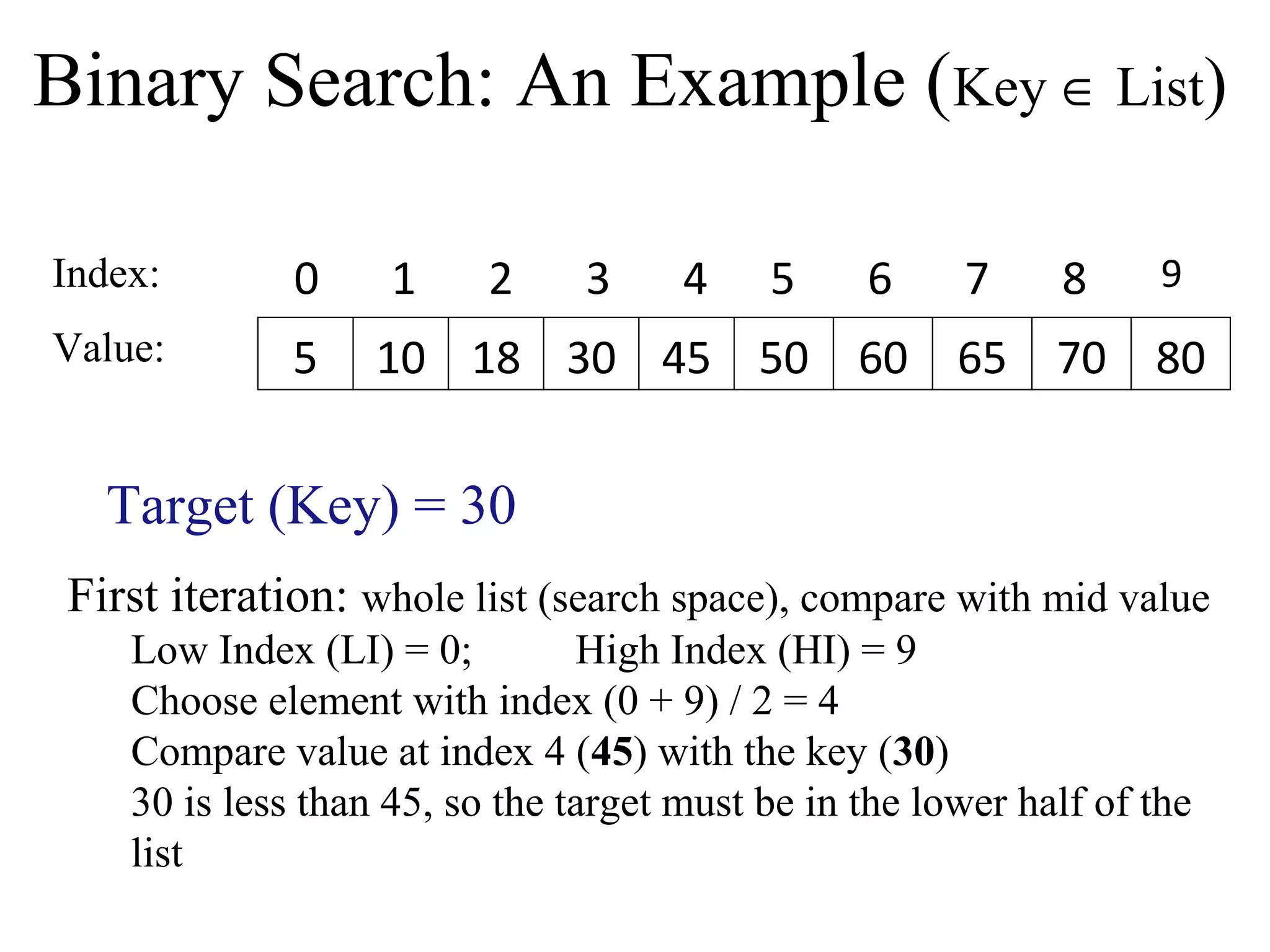
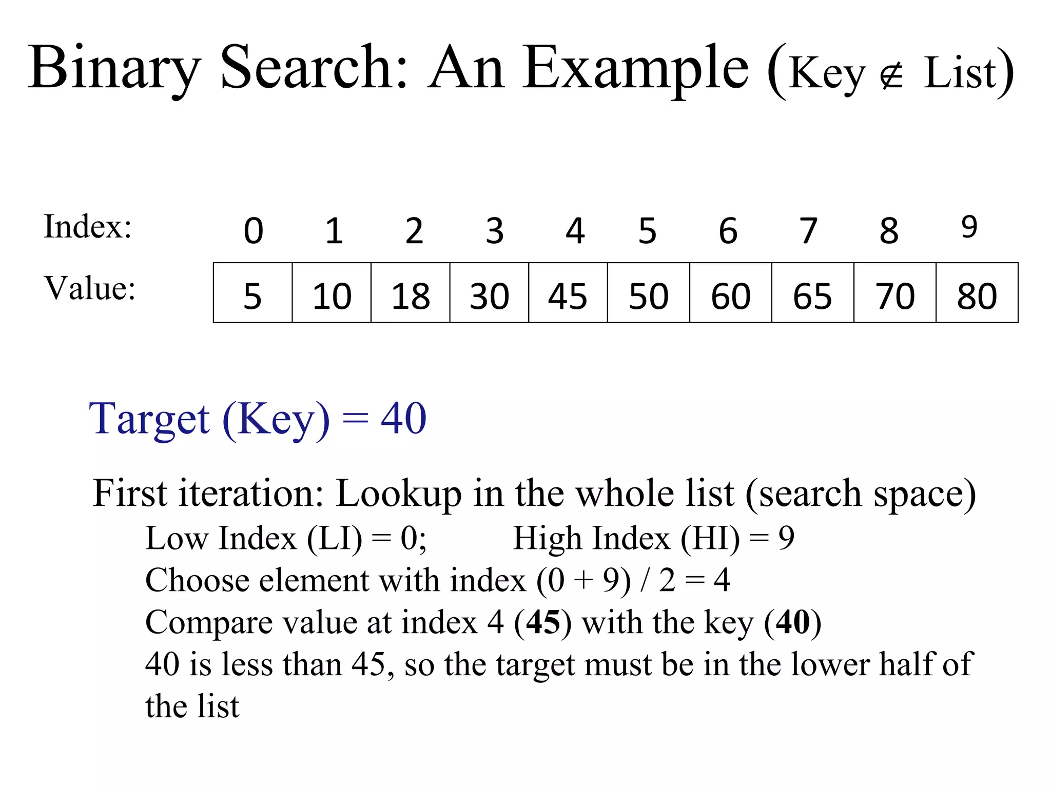
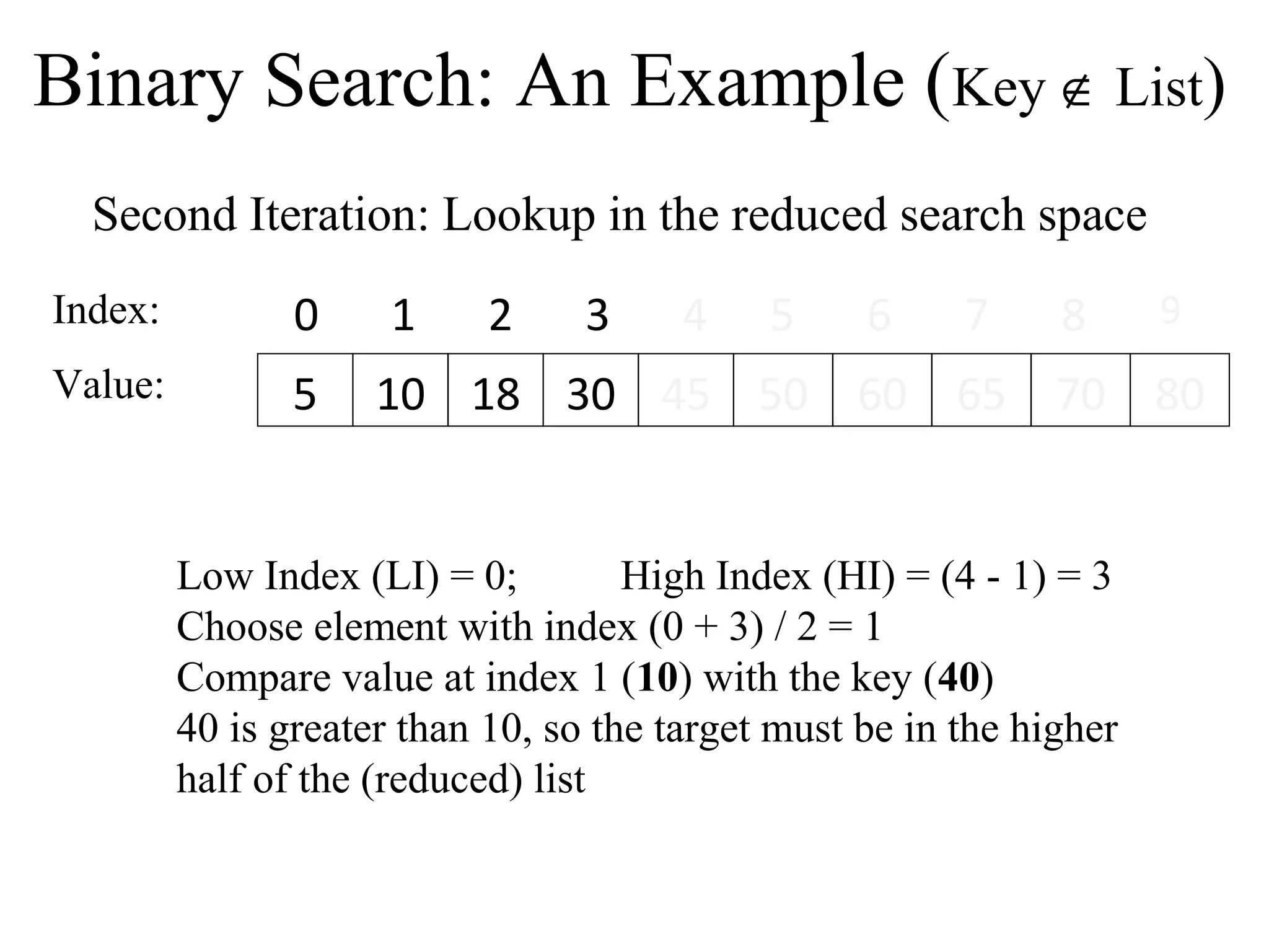
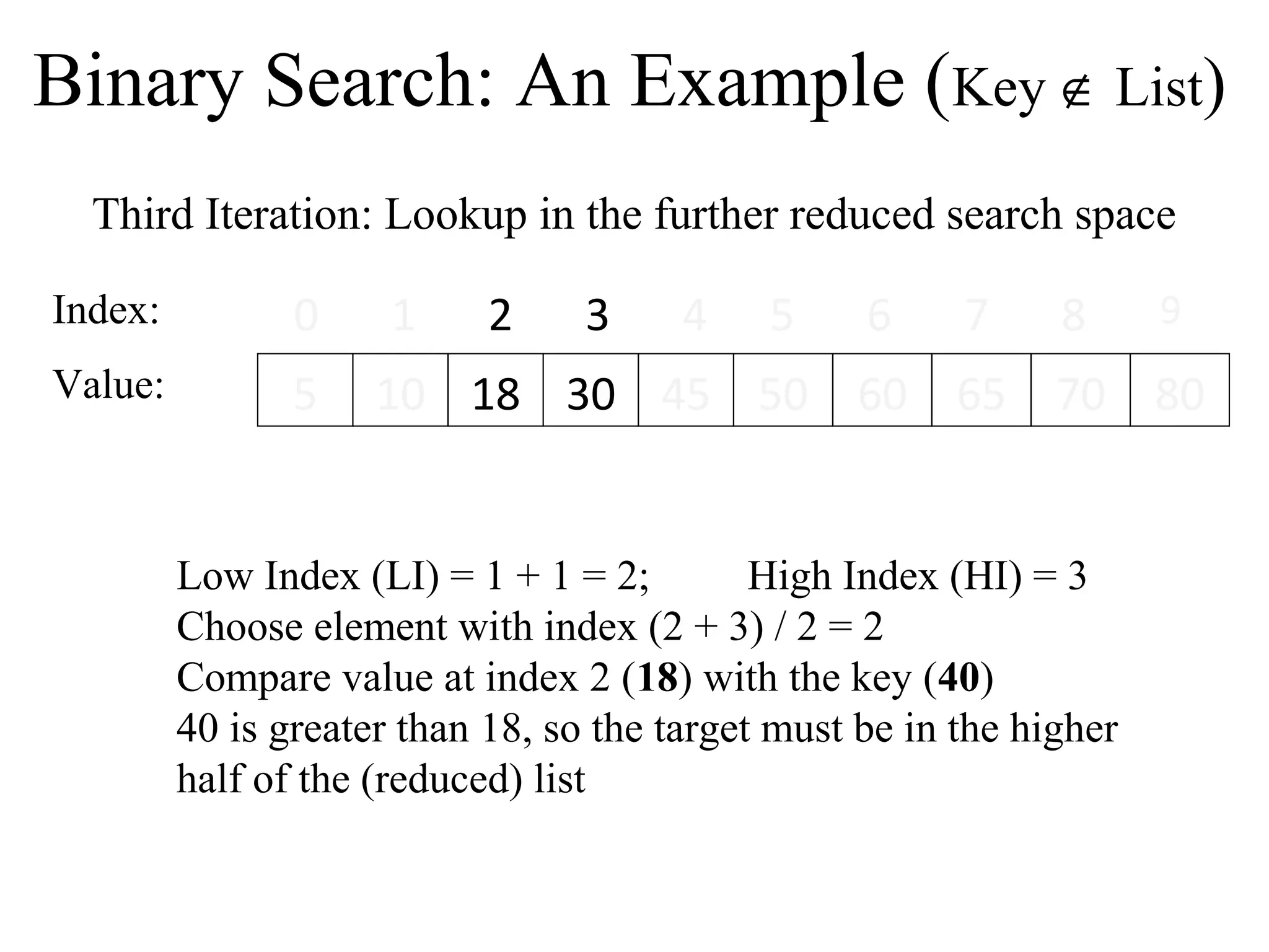
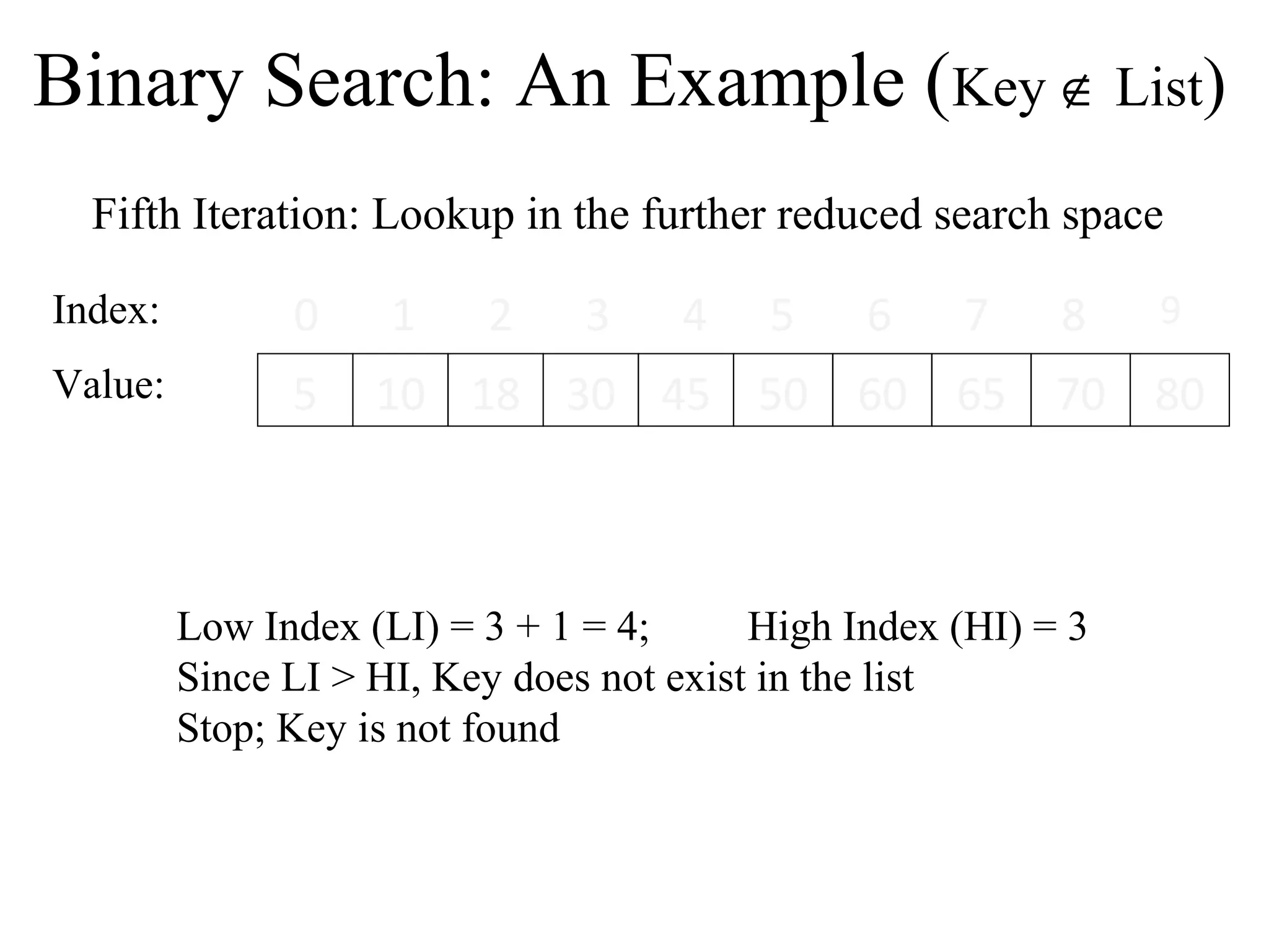
![Binary Search Algorithm: Informal
Middle (LI + HI) / 2
One of the three possibilities
Key is equal to List[Middle]
o success and stop
Key is less than List[Middle]
o Key should be in the left half of List, or it does not exist
Key is greater than List[Middle]
o Key should be in the right half of List, or it does not exist
Termination Condition
List[Middle] is equal to Key (success) OR LI > HI
(Failure)](https://image.slidesharecdn.com/part3arraysandsearchingalgorithms-140828232254-phpapp02/85/Data-Structures-Part3-arrays-and-searching-algorithms-31-320.jpg)
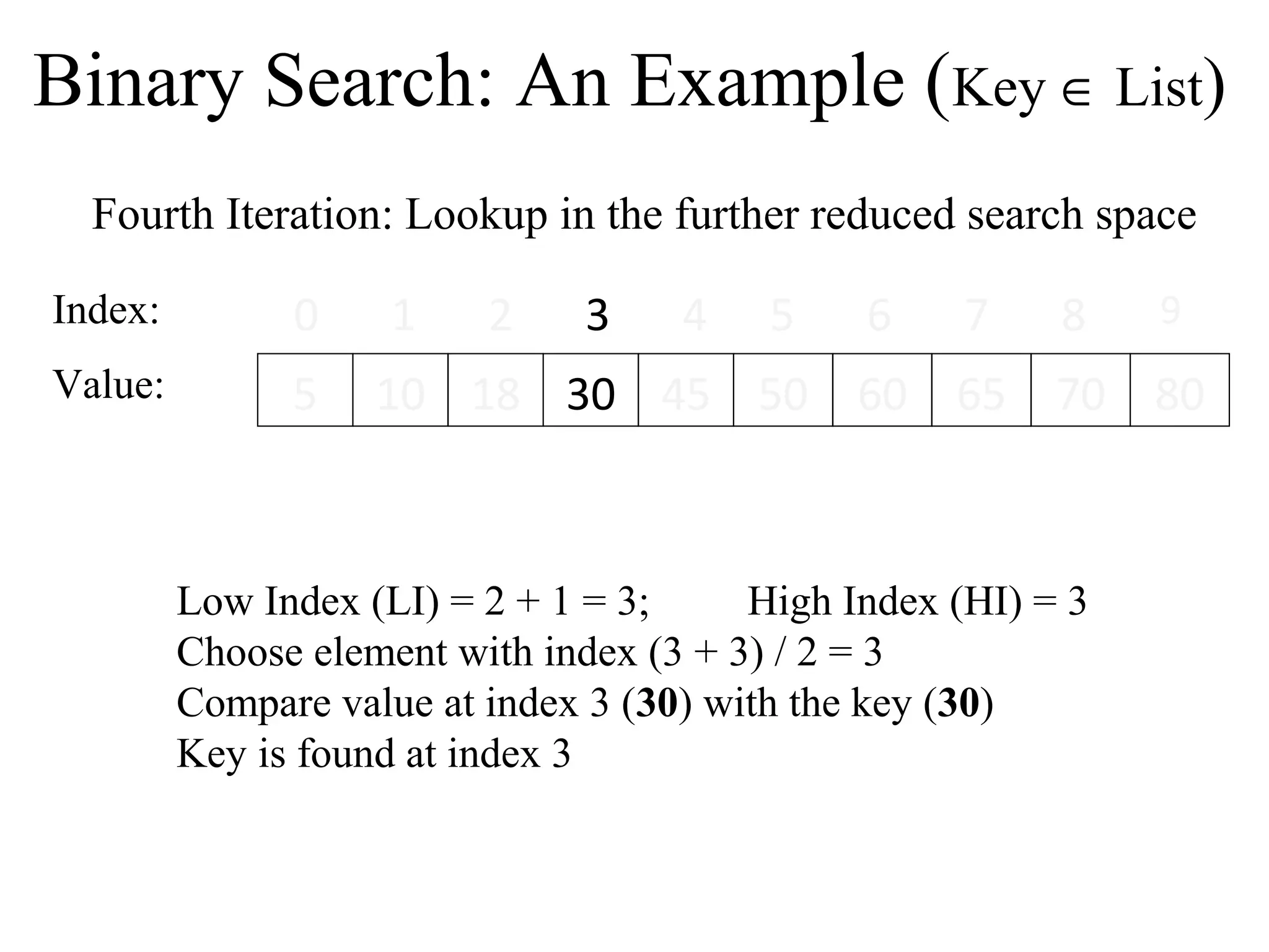
![Binary Search Algorithm
Input: Key, List
Initialisation: LI 0, HI SizeOf(List) – 1
Repeat steps 1 and 2 until LI > HI
1. Mid (LI + HI) / 2
2. If List[Mid] = Key then
Return Mid // success
Else If Key < List[Mid] then
HI Mid – 1
Else
LI Mid + 1
Return -1 // failure](https://image.slidesharecdn.com/part3arraysandsearchingalgorithms-140828232254-phpapp02/85/Data-Structures-Part3-arrays-and-searching-algorithms-32-320.jpg)


![Using Arrays
Array_name[index]
For example, in Java
System.out.println(data[4]) will display
0
data[3] = 99 will replace -3 with 99](https://image.slidesharecdn.com/part3arraysandsearchingalgorithms-140828232254-phpapp02/75/Data-Structures-Part3-arrays-and-searching-algorithms-8-2048.jpg)
![Some more concepts
data[ -1 ] always illegal
data[ 10 ] illegal (10 > upper bound)
data[ 1.5 ] always illegal
data[ 0 ] always OK
data[ 9 ] OK
Q. What will be the output of?
1.data[5] + 10
2.data[3] = data[3] + 10](https://image.slidesharecdn.com/part3arraysandsearchingalgorithms-140828232254-phpapp02/75/Data-Structures-Part3-arrays-and-searching-algorithms-9-2048.jpg)
![Two dimensional Arrays
Let, the name of the two dimensional array is M
20 25 60 40
30 15 70 90
Two indices/subscripts are required (row,
column)
First element is at row 0, column 0
M0,0 or M(0, 0) or M[0][0] (more common)
What is: M[1][2]? M[3][4]?](https://image.slidesharecdn.com/part3arraysandsearchingalgorithms-140828232254-phpapp02/75/Data-Structures-Part3-arrays-and-searching-algorithms-11-2048.jpg)
![Array Operations
Indexing: inspect or update an element using its index.
Performance is very fast O(1)
randomNumber = numbers[5];
numbers[20000] = 100;
Insertion: add an element at certain index
– Start: very slow O(n) because of shift
– End : very fast O(1) because no need to shift
Removal: remove an element at certain index
– Start: very slow O(n) because of shift
– End : very fast O(1) because no need to shift
Search: performance depends on algorithm
1) Linear: slow O(n) 2) binary : O(log n)
Sort: performance depends on algorithm
1) Bubble: slow O(n2) 2) Selection: slow O(n2)
3) Insertion: slow O(n2) 4)Merge : O (n log n)](https://image.slidesharecdn.com/part3arraysandsearchingalgorithms-140828232254-phpapp02/75/Data-Structures-Part3-arrays-and-searching-algorithms-12-2048.jpg)
![One Dimensional Arrays in Java
To declare an array follow the type with (empty) []s
int[] grade; //or
int grade[]; //both declare an int array
In Java arrays are objects so must be created with the new
keyword
To create an array of ten integers:
int[] grade = new int[10];
Note that the array size has to be specified, although it can be
specified with a variable at run-time](https://image.slidesharecdn.com/part3arraysandsearchingalgorithms-140828232254-phpapp02/75/Data-Structures-Part3-arrays-and-searching-algorithms-13-2048.jpg)
![Arrays in Java
When the array is created memory is reserved for its contents
Initialization lists can be used to specify the initial values of an
array, in which case the new operator is not used
int[] grade = {87, 93, 35}; //array of 3 ints
To find the length of an array use its .length property
int numGrades = grade.length; //note: not .length()!!](https://image.slidesharecdn.com/part3arraysandsearchingalgorithms-140828232254-phpapp02/75/Data-Structures-Part3-arrays-and-searching-algorithms-14-2048.jpg)
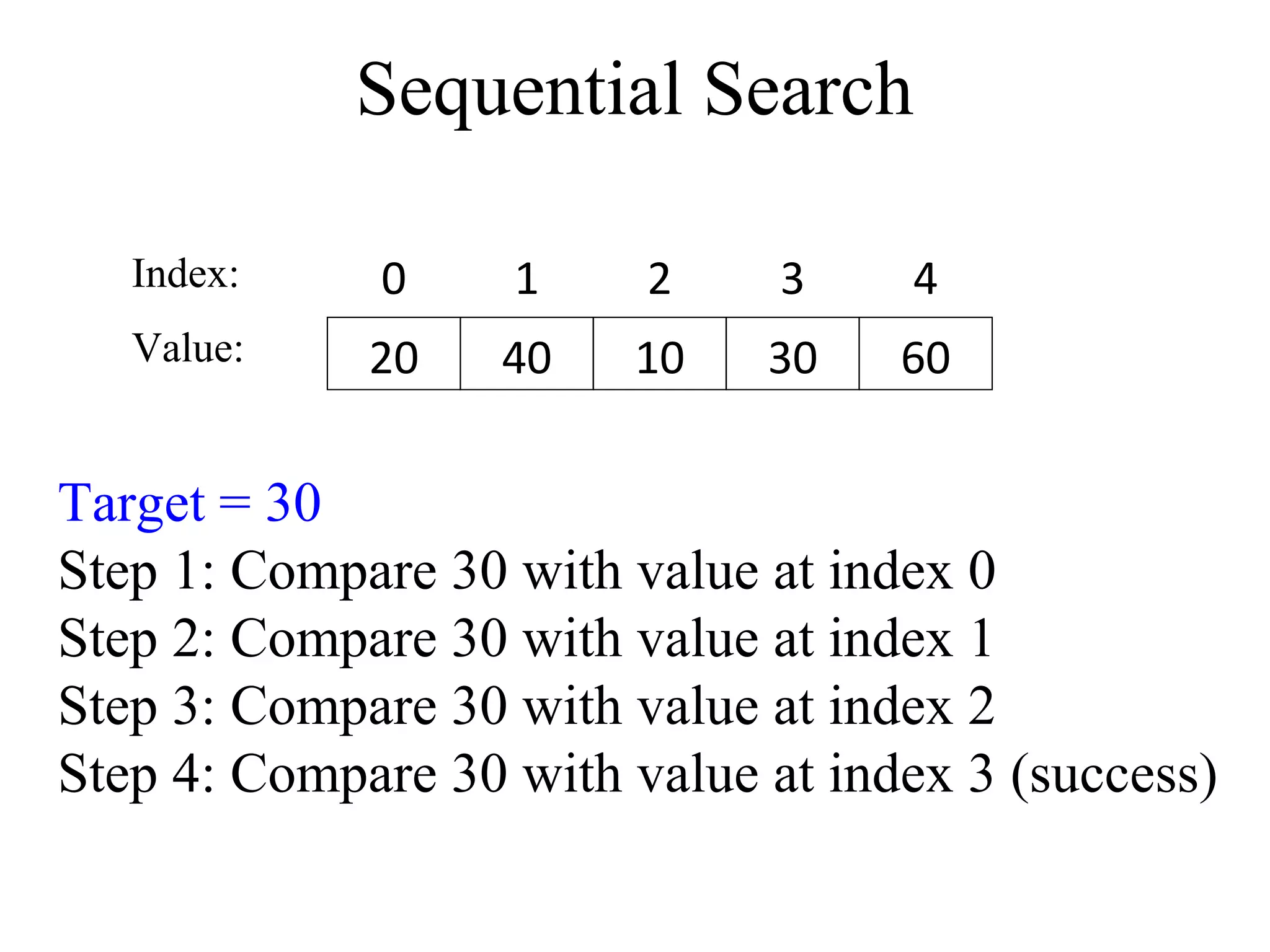
![Sequential Search Algorithm
Given: A list of N elements, and the target
1. index 0
2. Repeat steps 3 to 5
3. Compare target with list[index]
4. if target = list[index] then
return index // success
else if index >= N - 1
return -1 // failure
5. index index + 1](https://image.slidesharecdn.com/part3arraysandsearchingalgorithms-140828232254-phpapp02/75/Data-Structures-Part3-arrays-and-searching-algorithms-20-2048.jpg)


![Binary Search Algorithm: Informal
Middle (LI + HI) / 2
One of the three possibilities
Key is equal to List[Middle]
o success and stop
Key is less than List[Middle]
o Key should be in the left half of List, or it does not exist
Key is greater than List[Middle]
o Key should be in the right half of List, or it does not exist
Termination Condition
List[Middle] is equal to Key (success) OR LI > HI
(Failure)](https://image.slidesharecdn.com/part3arraysandsearchingalgorithms-140828232254-phpapp02/75/Data-Structures-Part3-arrays-and-searching-algorithms-31-2048.jpg)
![Binary Search Algorithm
Input: Key, List
Initialisation: LI 0, HI SizeOf(List) – 1
Repeat steps 1 and 2 until LI > HI
1. Mid (LI + HI) / 2
2. If List[Mid] = Key then
Return Mid // success
Else If Key < List[Mid] then
HI Mid – 1
Else
LI Mid + 1
Return -1 // failure](https://image.slidesharecdn.com/part3arraysandsearchingalgorithms-140828232254-phpapp02/75/Data-Structures-Part3-arrays-and-searching-algorithms-32-2048.jpg)


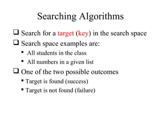
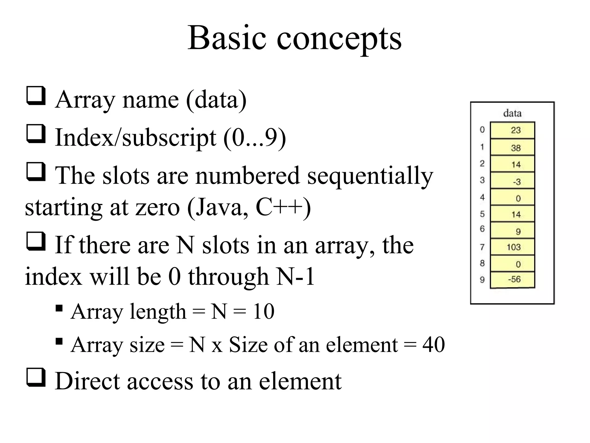
This document discusses arrays and searching algorithms. It begins by defining data structures and describing different types, including arrays. Arrays are introduced as a way to store multiple values of the same type in contiguous memory locations. Sequential and binary search algorithms are then described. Sequential search has linear time complexity, while binary search has logarithmic time complexity when used on a sorted array. Key concepts of arrays like indexing, dimensionality, and operations are also covered. The document concludes by looking ahead to sorting algorithms to be discussed in the next week.


![Data Structures - Lecture 3 [Arrays]](https://cdn.slidesharecdn.com/ss_thumbnails/lecture-3arrays-141224100714-conversion-gate01-thumbnail.jpg?width=600ounds&width=560&fit=bounds)


