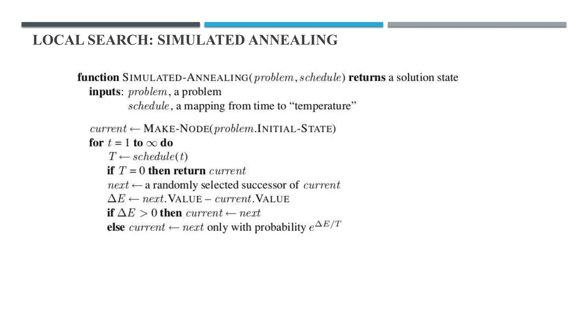
KEMBAR78
Searching Algorithms AI and Machine Learning | PPTX
LOCAL SEARCH
DR SURESH KUMAR
LOCAL SEARCH
 The search algorithms explore search spaces systematically by keeping one or more
paths in memory and by recording which alternatives have been explored at each
point along the path.
 When a goal is found, the path to that goal also constitutes a solution to the problem.
 In many problems, however, the path to the goal is irrelevant. For example, in the 8-
queens problem, what matters is the final configuration of queens, not the order in
which they are added.
 The same general property holds for many important applications such as integrated-
circuit design, factory-floor layout, job-shop scheduling, automatic programming,
telecommunications network optimization, vehicle routing, and portfolio
management.
LOCAL SEARCH
 If the path to the goal is irrelevant, we might consider a different class of algorithms,
ones that do not worry about paths at all.
 Local search algorithms operate using a single current node (rather than multiple paths)
and generally move only to neighbors of that node. Typically, the paths followed by the
search are not retained.
 Although local search algorithms are not systematic, they have two key advantages:
 They use very little memory, usually a constant amount
 They can often find reasonable solutions in large or infinite (continuous) state spaces
for which systematic algorithms are unsuitable.
 In addition to finding goals, local search algorithms are useful for solving pure
optimization problems, in which the aim is to find the best state according to an objective
function.
LOCAL SEARCH: HILL CLIMBING SEARCH
 It is simply a loop that continually moves in the direction of increasing value,
that is, uphill.
 It terminates when it reaches a “peak” where no neighbor has a higher value.
 The algorithm does not maintain a search tree, so the data structure for the
current node need only record the state and the value of the objective function.
 Hill climbing does not look ahead beyond the immediate neighbors of the
current state. This resembles trying to find the top of Mount Everest in a thick
fog while suffering from amnesia.
LOCAL SEARCH: HILL CLIMBING SEARCH
 Consider 8-queens problem to understand the Hill Climbing search.
 Local search algorithms typically use a complete-state formulation, where each state has 8
queens on the board, one per column.
 The successors of a state are all possible states generated by moving a single queen to another
square in the same column (so each state has 8 × 7 = 56 successors).
 The heuristic cost function h is the number of pairs of queens that are attacking each other,
either directly or indirectly.
 The global minimum of this function is zero, which occurs only at perfect solutions. Figure
(a) shows a state with h = 17.
 The figure also shows the values of all its successors, with the best successors having h = 12.
 Hill-climbing algorithms typically choose randomly among the set of best successors if there
is more than one.
LOCAL SEARCH: HILL CLIMBING SEARCH
LOCAL SEARCH: HILL CLIMBING SEARCH STATE SPACE
 A state-space diagram consists of various regions that can be explained as follows;
 Local maximum: A local maximum is a solution that surpasses other neighboring solutions
or states but is not the best possible solution. This will lead to the hill-climbing process’s
termination, even though this is not the best possible solution.
 Global maximum: This is the best possible solution achieved by the algorithm.
 Current state: This is the existing or present state.
 Flat local maximum: This is a flat region where the neighboring solutions attain the same
value. This makes it difficult for the algorithm to choose the best direction.
 Shoulder: This is a plateau whose edge is stretching upwards.
 When algorithm gets stuck in situation where no neighbor is at highest value or all are of
same value, the algorithm increases step size to get out of the situation.
LOCAL SEARCH: HILL CLIMBING SEARCH TYPES
 Simple hill Climbing: It only checks its one successor state, and if it finds better than the current state,
then move else be in the same state. This algorithm has the following features:
 Less time consuming
 Less optimal solution and the solution is not guaranteed
 Algorithm for Simple Hill Climbing:
 Step 1: Evaluate the initial state, if it is goal state then return success and Stop.
 Step 2: Loop Until a solution is found or there is no new operator left to apply.
 Step 3: Select and apply an operator to the current state.
 Step 4: Check new state:
 If it is goal state, then return success and quit.
 Else if it is better than the current state then assign new state as a current state.
 Else if not better than the current state, then return to step2.
 Step 5: Exit.
LOCAL SEARCH: HILL CLIMBING SEARCH TYPES
 Steepest-Ascent hill climbing: This examines all the neighboring nodes of the current state and selects
one neighbor node which is closest to the goal state. This algorithm consumes more time as it searches for
multiple neighbors.
 Algorithm for Steepest-Ascent Hill Climbing:
 Step 1: Evaluate the initial state, if it is goal state then return success and stop, else make current state as initial state.
 Step 2: Loop until a solution is found or the current state does not change.
 Step 3: Let SUCCESSOR be a state such that any successor of the current state will be better than it.
 Step 4: For each operator that applies to the current state:
 Apply the new operator and generate a new state.
 Evaluate the new state.
 If it is goal state, then return it and quit, else compare it to the SUCCESSOR.
 If it is better than SUCCESSOR, then set new state as SUCCESSOR.
 If the SUCC is better than the current state, then set current state to SUCCESSOR.
 Step 5: Exit.
LOCAL SEARCH: HILL CLIMBING SEARCH TYPES
 Stochastic hill climbing: This does not examine for all its neighbor before moving. Rather, this search
algorithm selects one neighbor node at random and decides whether to choose it as a current state or
examine another state. This is a good strategy when a state has many (e.g., thousands) of successors.
 Algorithm for Stochastic Hill Climbing:
 Step 1: Evaluate the initial state, if it is goal state then return success and stop, else make current state as initial state.
 Step 2: Loop until current state is a solution or the current state does not change or have no neighbors.
 Step 3: neighbor = pick a random neighbor of current state
 Step 4: If neighbor.value>current state.value set neighbor as current state
 Step 4: Exit.
LOCAL SEARCH: SIMULATED ANNEALING
 A hill-climbing algorithm that never makes “downhill” moves toward states with lower value (or
higher cost) is guaranteed to be incomplete, because it can get stuck on a local maximum.
 In contrast, a purely random walk—that is, moving to a successor chosen at random from the set
of successors—is complete but extremely inefficient.
 Therefore, it seems reasonable to try to combine hill climbing with a random walk in some way
that yields both efficiency and completeness. Simulated annealing is such an algorithm.
 It is useful in finding global optima in the presence of large numbers of local optima.
 In metallurgy, annealing is the process used to temper or harden metals and glass by heating them
to a high temperature and then gradually cooling them, thus allowing the material to reach a low-
energy crystalline state.
 Simulated annealing uses the objective function of an optimization problem instead of the energy
of a material.
LOCAL SEARCH: SIMULATED ANNEALING
 The algorithm is basically hill-climbing except instead of picking the best move, it picks
a random move.
 If the selected move improves the solution, then it is always accepted. Otherwise, the
algorithm makes the move anyway with some probability less than 1.
 The probability decreases exponentially with the “badness” of the move, which is the
amount ΔE by which the solution is worsened (i.e., energy is increased).
 Prob(accepting uphill move) = 1 - exp(ΔE / kT)
 The probability also decreases as the “temperature” T goes down: “bad” moves are more
likely to be allowed at the start when T is high, and they become more unlikely as T
decreases.
 If the schedule lowers T slowly enough, the algorithm will find a global optimum with
probability approaching 1.
LOCAL SEARCH: SIMULATED ANNEALING
LOCAL SEARCH: LOCAL BEAM
 Keeping just one node in memory might seem to be an extreme reaction to the problem of
memory limitations.
 The local beam search algorithm keeps track of k states rather than just one. It begins with k
randomly generated states. At each step, all the successors of all k states are generated.
 If any one is a goal, the algorithm halts. Otherwise, it selects the k best successors from the
complete list and repeats.
 In its simplest form, local beam search can suffer from a lack of diversity among the k states—
they can quickly become concentrated in a small region of the state space, making the search
little more than an expensive version of hill climbing.
 A variant called stochastic beam search, analogous to stochastic hill climbing, helps alleviate this
problem. Instead of choosing the best k from the the pool of candidate successors, stochastic
beam search chooses k successors at random, with the probability of choosing a given successor
being an increasing function of its value.
LOCAL SEARCH: GENETIC ALGORITHM
 A genetic algorithm (or GA) is a variant of stochastic beam search in which successor states are
generated by combining two parent states rather than by modifying a single state.
 GAs begin with a set of k randomly generated states, called the population. Each state, or
individual, is represented as a string over a finite alphabet—most commonly, a string of 0s and
1s.
 Each state is rated by the objective function, or (in GA terminology) the fitness function.
 A fitness function should return higher values for better states.
 Two pairs are selected at random for reproduction, in accordance with the probability or fitness
function. For each pair to be mated, a crossover point is chosen randomly.
 Finally, each offspring is subject to random mutation with a small independent probability.
 The process is repeated to get best state or outcome same as the goal or near to the goal.
LOCAL SEARCH: GENETIC ALGORITHM
 Initialization of Population(Coding)
 Every gene represents a parameter (variables) in the solution. This collection of parameters that
forms the solution is the chromosome. Therefore, the population is a collection of
chromosomes.
 Order of genes on the chromosome matters.
 Chromosomes are often depicted in binary as 0’s and 1’s, but other encoding are also possible.
 Fitness Function
 We have to select the best ones to reproduce offspring out of the available chromosomes, so
each chromosome is given a fitness value.
 The fitness score helps to select the individuals who will be used for reproduction.
LOCAL SEARCH: GENETIC ALGORITHM
 Selection
 This phase’s main goal is to find the region where possibility of getting the best solution is
higher.
 Inspiration for this is from the survival of the fittest.
 It should be a balance between exploration and exploitation of search space.
 Too strong fitness selection bias can lead to sub-optimal solutions.
 Too little fitness bias selection results in an unfocused search.
 Thus, Fitness proportionate selection is used, also known as roulette wheel selection, as a
genetic operator used in genetic algorithms to select potentially useful recombination solutions.
LOCAL SEARCH: GENETIC ALGORITHM
 Reproduction
 Generation of off-springs happen in 2 ways: Crossover & Mutation
 Crossover is the most vital stage in the genetic algorithm. During which, a random point is
selected while mating a pair of parents to generate off-springs.
 There are 3 major types of crossover.
 Single Point Crossover: A point on both parents’ chromosomes is picked randomly and
designated a ‘crossover point’. Bits to the right of that point are exchanged between the two
parent chromosomes.
 Two-Point Crossover: Two crossover points are picked randomly from the parent chromosomes.
The bits in between the two points are swapped between the parent organisms.
 Uniform Crossover: In a uniform crossover, typically, each bit is chosen from either parent with
equal probability.
LOCAL SEARCH: GENETIC ALGORITHM
 Mutation: In a few new offspring formed, some of their genes can be subjected to a low
random probability mutation. This indicates that some of the bits in the bit chromosome can be
flipped. Mutation happens to take care of diversity among the population and stop premature
convergence.
 Convergence (when to stop): Few rules which are followed which tell when to stop is as
follows:
 When there is no improvement in the solution quality after completing a certain number of
generations set beforehand.
 When a hard and fast range of generations and time is reached.
 Till an acceptable solution is obtained.
LOCAL SEARCH: GENETIC ALGORITHM

Searching Algorithms AI and Machine Learning

  • 1.
  • 2.
    LOCAL SEARCH  Thesearch algorithms explore search spaces systematically by keeping one or more paths in memory and by recording which alternatives have been explored at each point along the path.  When a goal is found, the path to that goal also constitutes a solution to the problem.  In many problems, however, the path to the goal is irrelevant. For example, in the 8- queens problem, what matters is the final configuration of queens, not the order in which they are added.  The same general property holds for many important applications such as integrated- circuit design, factory-floor layout, job-shop scheduling, automatic programming, telecommunications network optimization, vehicle routing, and portfolio management.
  • 3.
    LOCAL SEARCH  Ifthe path to the goal is irrelevant, we might consider a different class of algorithms, ones that do not worry about paths at all.  Local search algorithms operate using a single current node (rather than multiple paths) and generally move only to neighbors of that node. Typically, the paths followed by the search are not retained.  Although local search algorithms are not systematic, they have two key advantages:  They use very little memory, usually a constant amount  They can often find reasonable solutions in large or infinite (continuous) state spaces for which systematic algorithms are unsuitable.  In addition to finding goals, local search algorithms are useful for solving pure optimization problems, in which the aim is to find the best state according to an objective function.
  • 4.
    LOCAL SEARCH: HILLCLIMBING SEARCH  It is simply a loop that continually moves in the direction of increasing value, that is, uphill.  It terminates when it reaches a “peak” where no neighbor has a higher value.  The algorithm does not maintain a search tree, so the data structure for the current node need only record the state and the value of the objective function.  Hill climbing does not look ahead beyond the immediate neighbors of the current state. This resembles trying to find the top of Mount Everest in a thick fog while suffering from amnesia.
  • 5.
    LOCAL SEARCH: HILLCLIMBING SEARCH  Consider 8-queens problem to understand the Hill Climbing search.  Local search algorithms typically use a complete-state formulation, where each state has 8 queens on the board, one per column.  The successors of a state are all possible states generated by moving a single queen to another square in the same column (so each state has 8 × 7 = 56 successors).  The heuristic cost function h is the number of pairs of queens that are attacking each other, either directly or indirectly.  The global minimum of this function is zero, which occurs only at perfect solutions. Figure (a) shows a state with h = 17.  The figure also shows the values of all its successors, with the best successors having h = 12.  Hill-climbing algorithms typically choose randomly among the set of best successors if there is more than one.
  • 6.
    LOCAL SEARCH: HILLCLIMBING SEARCH
  • 7.
    LOCAL SEARCH: HILLCLIMBING SEARCH STATE SPACE
  • 8.
    LOCAL SEARCH: HILLCLIMBING SEARCH STATE SPACE  A state-space diagram consists of various regions that can be explained as follows;  Local maximum: A local maximum is a solution that surpasses other neighboring solutions or states but is not the best possible solution. This will lead to the hill-climbing process’s termination, even though this is not the best possible solution.  Global maximum: This is the best possible solution achieved by the algorithm.  Current state: This is the existing or present state.  Flat local maximum: This is a flat region where the neighboring solutions attain the same value. This makes it difficult for the algorithm to choose the best direction.  Shoulder: This is a plateau whose edge is stretching upwards.  When algorithm gets stuck in situation where no neighbor is at highest value or all are of same value, the algorithm increases step size to get out of the situation.
  • 9.
    LOCAL SEARCH: HILLCLIMBING SEARCH TYPES  Simple hill Climbing: It only checks its one successor state, and if it finds better than the current state, then move else be in the same state. This algorithm has the following features:  Less time consuming  Less optimal solution and the solution is not guaranteed  Algorithm for Simple Hill Climbing:  Step 1: Evaluate the initial state, if it is goal state then return success and Stop.  Step 2: Loop Until a solution is found or there is no new operator left to apply.  Step 3: Select and apply an operator to the current state.  Step 4: Check new state:  If it is goal state, then return success and quit.  Else if it is better than the current state then assign new state as a current state.  Else if not better than the current state, then return to step2.  Step 5: Exit.
  • 10.
    LOCAL SEARCH: HILLCLIMBING SEARCH TYPES  Steepest-Ascent hill climbing: This examines all the neighboring nodes of the current state and selects one neighbor node which is closest to the goal state. This algorithm consumes more time as it searches for multiple neighbors.  Algorithm for Steepest-Ascent Hill Climbing:  Step 1: Evaluate the initial state, if it is goal state then return success and stop, else make current state as initial state.  Step 2: Loop until a solution is found or the current state does not change.  Step 3: Let SUCCESSOR be a state such that any successor of the current state will be better than it.  Step 4: For each operator that applies to the current state:  Apply the new operator and generate a new state.  Evaluate the new state.  If it is goal state, then return it and quit, else compare it to the SUCCESSOR.  If it is better than SUCCESSOR, then set new state as SUCCESSOR.  If the SUCC is better than the current state, then set current state to SUCCESSOR.  Step 5: Exit.
  • 11.
    LOCAL SEARCH: HILLCLIMBING SEARCH TYPES  Stochastic hill climbing: This does not examine for all its neighbor before moving. Rather, this search algorithm selects one neighbor node at random and decides whether to choose it as a current state or examine another state. This is a good strategy when a state has many (e.g., thousands) of successors.  Algorithm for Stochastic Hill Climbing:  Step 1: Evaluate the initial state, if it is goal state then return success and stop, else make current state as initial state.  Step 2: Loop until current state is a solution or the current state does not change or have no neighbors.  Step 3: neighbor = pick a random neighbor of current state  Step 4: If neighbor.value>current state.value set neighbor as current state  Step 4: Exit.
  • 12.
    LOCAL SEARCH: SIMULATEDANNEALING  A hill-climbing algorithm that never makes “downhill” moves toward states with lower value (or higher cost) is guaranteed to be incomplete, because it can get stuck on a local maximum.  In contrast, a purely random walk—that is, moving to a successor chosen at random from the set of successors—is complete but extremely inefficient.  Therefore, it seems reasonable to try to combine hill climbing with a random walk in some way that yields both efficiency and completeness. Simulated annealing is such an algorithm.  It is useful in finding global optima in the presence of large numbers of local optima.  In metallurgy, annealing is the process used to temper or harden metals and glass by heating them to a high temperature and then gradually cooling them, thus allowing the material to reach a low- energy crystalline state.  Simulated annealing uses the objective function of an optimization problem instead of the energy of a material.
  • 13.
    LOCAL SEARCH: SIMULATEDANNEALING  The algorithm is basically hill-climbing except instead of picking the best move, it picks a random move.  If the selected move improves the solution, then it is always accepted. Otherwise, the algorithm makes the move anyway with some probability less than 1.  The probability decreases exponentially with the “badness” of the move, which is the amount ΔE by which the solution is worsened (i.e., energy is increased).  Prob(accepting uphill move) = 1 - exp(ΔE / kT)  The probability also decreases as the “temperature” T goes down: “bad” moves are more likely to be allowed at the start when T is high, and they become more unlikely as T decreases.  If the schedule lowers T slowly enough, the algorithm will find a global optimum with probability approaching 1.
  • 14.
  • 15.
    LOCAL SEARCH: LOCALBEAM  Keeping just one node in memory might seem to be an extreme reaction to the problem of memory limitations.  The local beam search algorithm keeps track of k states rather than just one. It begins with k randomly generated states. At each step, all the successors of all k states are generated.  If any one is a goal, the algorithm halts. Otherwise, it selects the k best successors from the complete list and repeats.  In its simplest form, local beam search can suffer from a lack of diversity among the k states— they can quickly become concentrated in a small region of the state space, making the search little more than an expensive version of hill climbing.  A variant called stochastic beam search, analogous to stochastic hill climbing, helps alleviate this problem. Instead of choosing the best k from the the pool of candidate successors, stochastic beam search chooses k successors at random, with the probability of choosing a given successor being an increasing function of its value.
  • 16.
    LOCAL SEARCH: GENETICALGORITHM  A genetic algorithm (or GA) is a variant of stochastic beam search in which successor states are generated by combining two parent states rather than by modifying a single state.  GAs begin with a set of k randomly generated states, called the population. Each state, or individual, is represented as a string over a finite alphabet—most commonly, a string of 0s and 1s.  Each state is rated by the objective function, or (in GA terminology) the fitness function.  A fitness function should return higher values for better states.  Two pairs are selected at random for reproduction, in accordance with the probability or fitness function. For each pair to be mated, a crossover point is chosen randomly.  Finally, each offspring is subject to random mutation with a small independent probability.  The process is repeated to get best state or outcome same as the goal or near to the goal.
  • 18.
    LOCAL SEARCH: GENETICALGORITHM  Initialization of Population(Coding)  Every gene represents a parameter (variables) in the solution. This collection of parameters that forms the solution is the chromosome. Therefore, the population is a collection of chromosomes.  Order of genes on the chromosome matters.  Chromosomes are often depicted in binary as 0’s and 1’s, but other encoding are also possible.  Fitness Function  We have to select the best ones to reproduce offspring out of the available chromosomes, so each chromosome is given a fitness value.  The fitness score helps to select the individuals who will be used for reproduction.
  • 19.
    LOCAL SEARCH: GENETICALGORITHM  Selection  This phase’s main goal is to find the region where possibility of getting the best solution is higher.  Inspiration for this is from the survival of the fittest.  It should be a balance between exploration and exploitation of search space.  Too strong fitness selection bias can lead to sub-optimal solutions.  Too little fitness bias selection results in an unfocused search.  Thus, Fitness proportionate selection is used, also known as roulette wheel selection, as a genetic operator used in genetic algorithms to select potentially useful recombination solutions.
  • 20.
    LOCAL SEARCH: GENETICALGORITHM  Reproduction  Generation of off-springs happen in 2 ways: Crossover & Mutation  Crossover is the most vital stage in the genetic algorithm. During which, a random point is selected while mating a pair of parents to generate off-springs.  There are 3 major types of crossover.  Single Point Crossover: A point on both parents’ chromosomes is picked randomly and designated a ‘crossover point’. Bits to the right of that point are exchanged between the two parent chromosomes.  Two-Point Crossover: Two crossover points are picked randomly from the parent chromosomes. The bits in between the two points are swapped between the parent organisms.  Uniform Crossover: In a uniform crossover, typically, each bit is chosen from either parent with equal probability.
  • 21.
    LOCAL SEARCH: GENETICALGORITHM  Mutation: In a few new offspring formed, some of their genes can be subjected to a low random probability mutation. This indicates that some of the bits in the bit chromosome can be flipped. Mutation happens to take care of diversity among the population and stop premature convergence.  Convergence (when to stop): Few rules which are followed which tell when to stop is as follows:  When there is no improvement in the solution quality after completing a certain number of generations set beforehand.  When a hard and fast range of generations and time is reached.  Till an acceptable solution is obtained.
  • 22.
  • 23.