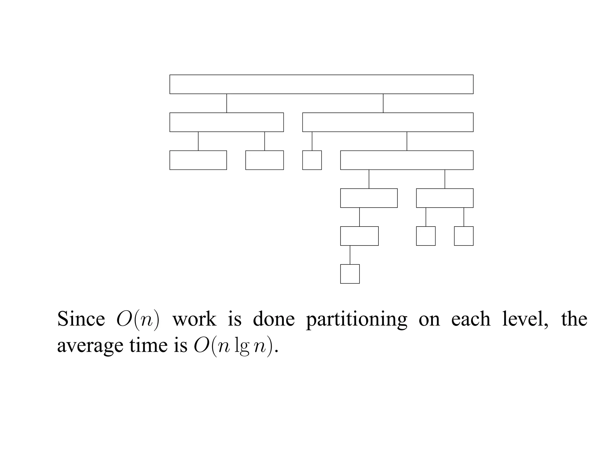
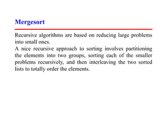
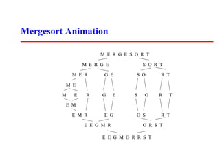
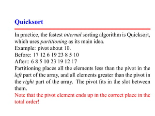
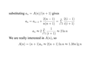
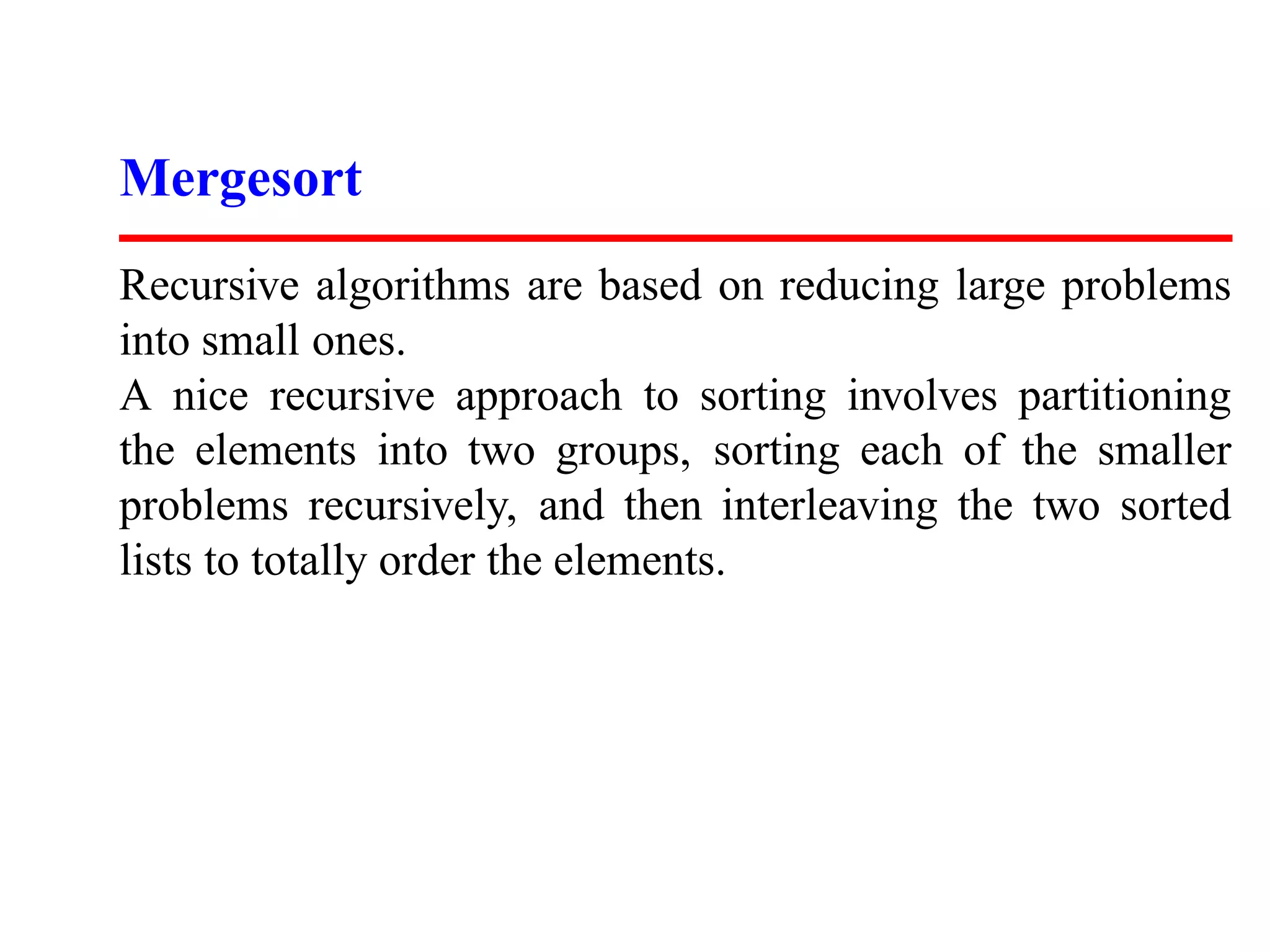
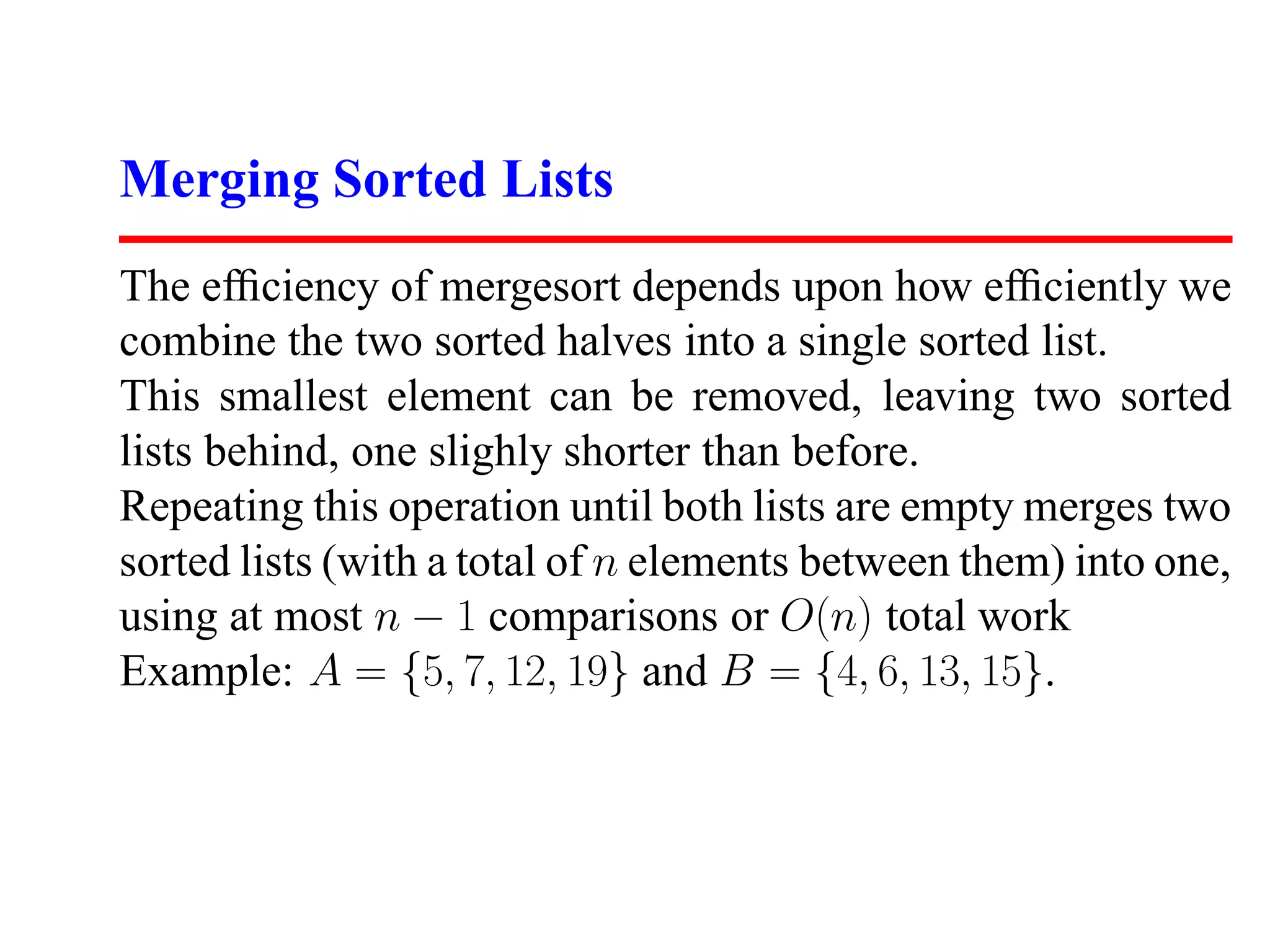
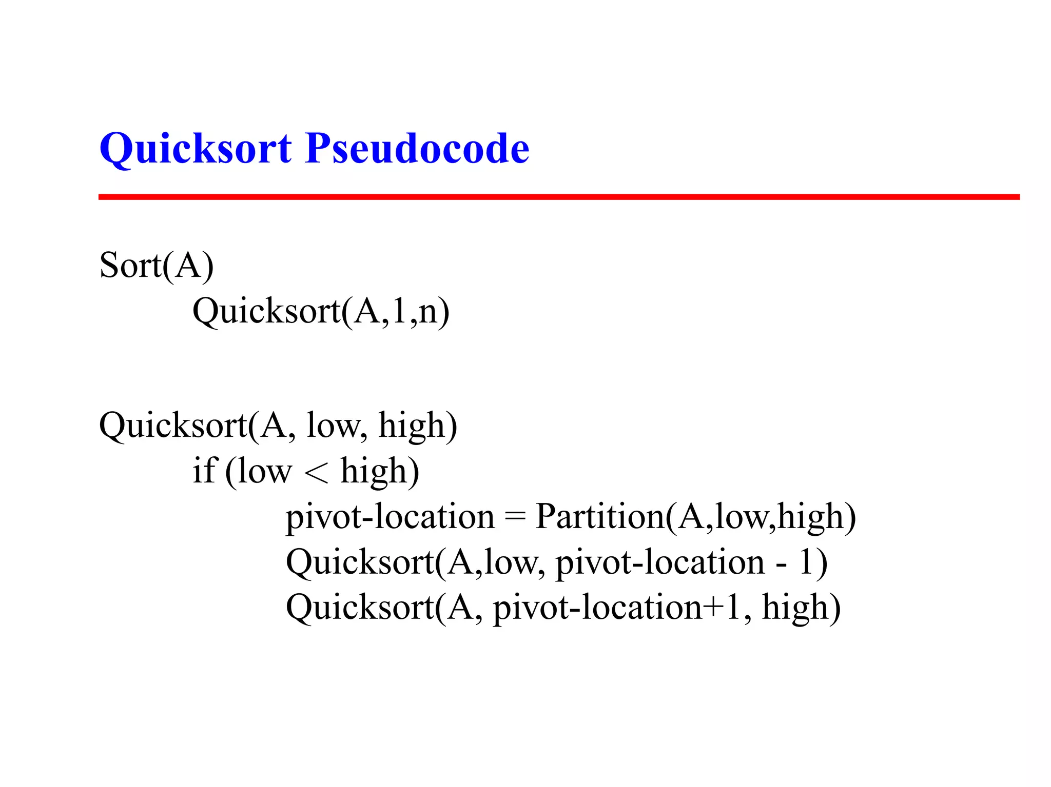
KEMBAR78
Skiena algorithm 2007 lecture08 quicksort | PDF
Lecture 8:
     Mergesort / Quicksort
         Steven Skiena

Department of Computer Science
 State University of New York
 Stony Brook, NY 11794–4400

http://www.cs.sunysb.edu/∼skiena
Problem of the Day
Given an array-based heap on n elements and a real number
x, efficiently determine whether the kth smallest in the heap
is greater than or equal to x. Your algorithm should be O(k)
in the worst-case, independent of the size of the heap. Hint:
you not have to find the kth smallest element; you need only
determine its relationship to x.
Solution
Mergesort
Recursive algorithms are based on reducing large problems
into small ones.
A nice recursive approach to sorting involves partitioning
the elements into two groups, sorting each of the smaller
problems recursively, and then interleaving the two sorted
lists to totally order the elements.
Mergesort Implementation

mergesort(item type s[], int low, int high)
{
     int i; (* counter *)
     int middle; (* index of middle element *)

     if (low < high) {
            middle = (low+high)/2;
            mergesort(s,low,middle);
            mergesort(s,middle+1,high);

           merge(s, low, middle, high);
     }
}
Mergesort Animation

                      M E R G E S O R T

                M E R G E            S O R T

            M E R      G E        S O      R T

         M E

        M   E    R    G     E    S   O    R    T

         E M

            E M R      E G        O S      R T

                E E G M R            O R S T

                      E E G M O R R S T
Merging Sorted Lists
The efficiency of mergesort depends upon how efficiently we
combine the two sorted halves into a single sorted list.
This smallest element can be removed, leaving two sorted
lists behind, one slighly shorter than before.
Repeating this operation until both lists are empty merges two
sorted lists (with a total of n elements between them) into one,
using at most n − 1 comparisons or O(n) total work
Example: A = {5, 7, 12, 19} and B = {4, 6, 13, 15}.
Buffering
Although mergesort is O(n lg n), it is inconvenient to
implement with arrays, since we need extra space to merge.
the lists.
Merging (4, 5, 6) and (1, 2, 3) would overwrite the first three
elements if they were packed in an array.
Writing the merged list to a buffer and recopying it uses extra
space but not extra time (in the big Oh sense).
External Sorting
Which O(n log n) algorithm you use for sorting doesn’t
matter much until n is so big the data does not fit in memory.
Mergesort proves to be the basis for the most efficient
external sorting programs.
Disks are much slower than main memory, and benefit from
algorithms that read and write data in long streams – not
random access.
Divide and Conquer
Divide and conquer is an important algorithm design tech-
nique using in mergesort, binary search the fast Fourier trans-
form (FFT), and Strassen’s matrix multiplication algorithm.
We divide the problem into two smaller subproblems, solve
each recursively, and then meld the two partial solutions into
one solution for the full problem.
When merging takes less time than solving the two subprob-
lems, we get an efficient algorithm.
Quicksort
In practice, the fastest internal sorting algorithm is Quicksort,
which uses partitioning as its main idea.
Example: pivot about 10.
Before: 17 12 6 19 23 8 5 10
After:: 6 8 5 10 23 19 12 17
Partitioning places all the elements less than the pivot in the
left part of the array, and all elements greater than the pivot in
the right part of the array. The pivot fits in the slot between
them.
Note that the pivot element ends up in the correct place in the
total order!
Partitioning the Elements
We can partition an array about the pivot in one linear scan, by
maintaining three sections: < pivot, > pivot, and unexplored.
As we scan from left to right, we move the left bound to the
right when the element is less than the pivot, otherwise we
swap it with the rightmost unexplored element and move the
right bound one step closer to the left.
Why Partition?
Since the partitioning step consists of at most n swaps, takes
time linear in the number of keys. But what does it buy us?
1. The pivot element ends up in the position it retains in the
   final sorted order.
2. After a partitioning, no element flops to the other side of
   the pivot in the final sorted order.
Thus we can sort the elements to the left of the pivot and the
right of the pivot independently, giving us a recursive sorting
algorithm!
Quicksort Pseudocode

Sort(A)
      Quicksort(A,1,n)


Quicksort(A, low, high)
     if (low < high)
            pivot-location = Partition(A,low,high)
            Quicksort(A,low, pivot-location - 1)
            Quicksort(A, pivot-location+1, high)
Partition Implementation

Partition(A,low,high)
       pivot = A[low]
       leftwall = low
       for i = low+1 to high
              if (A[i] < pivot) then
                     leftwall = leftwall+1
                     swap(A[i],A[leftwall])
       swap(A[low],A[leftwall])
Quicksort Animation

               Q U I C K S O R T

               Q I C K S O R T U

               Q I C K O R S T U

               I C K O Q R S T U

               I C K O Q R S T U

               I C K O Q R S T U
Best Case for Quicksort
Since each element ultimately ends up in the correct position,
the algorithm correctly sorts. But how long does it take?
The best case for divide-and-conquer algorithms comes when
we split the input as evenly as possible. Thus in the best case,
each subproblem is of size n/2.
The partition step on each subproblem is linear in its size.
Thus the total effort in partitioning the 2k problems of size
n/2k is O(n).
Best Case Recursion Tree


The total partitioning on each level is O(n), and it take
lg n levels of perfect partitions to get to single element
subproblems. When we are down to single elements, the
problems are sorted. Thus the total time in the best case is
O(n lg n).
Worst Case for Quicksort
Suppose instead our pivot element splits the array as
unequally as possible. Thus instead of n/2 elements in the
smaller half, we get zero, meaning that the pivot element is
the biggest or smallest element in the array.
Now we have n−1 levels, instead of lg n, for a worst case time
of Θ(n2 ), since the first n/2 levels each have ≥ n/2 elements
to partition.
To justify its name, Quicksort had better be good in the
average case. Showing this requires some intricate analysis.
The divide and conquer principle applies to real life. If you
break a job into pieces, make the pieces of equal size!
Intuition: The Average Case for Quicksort
Suppose we pick the pivot element at random in an array of n
keys.

            1        n/4     n/2      3n/4     n


Half the time, the pivot element will be from the center half
of the sorted array.
Whenever the pivot element is from positions n/4 to 3n/4, the
larger remaining subarray contains at most 3n/4 elements.
How Many Good Partitions
If we assume that the pivot element is always in this range,
what is the maximum number of partitions we need to get
from n elements down to 1 element?
                (3/4)l · n = 1 −→ n = (4/3)l

                      lg n = l · lg(4/3)

Therefore l = lg(4/3) · lg(n) < 2 lg n good partitions suffice.
How Many Bad Partitions?
How often when we pick an arbitrary element as pivot will it
generate a decent partition?
Since any number ranked between n/4 and 3n/4 would make
a decent pivot, we get one half the time on average.
If we need 2 lg n levels of decent partitions to finish the job,
and half of random partitions are decent, then on average the
recursion tree to quicksort the array has ≈ 4 lg n levels.
Since O(n) work is done partitioning on each level, the
average time is O(n lg n).
Average-Case Analysis of Quicksort
To do a precise average-case analysis of quicksort, we
formulate a recurrence given the exact expected time T (n):
                  n 1
        T (n) =       (T (p − 1) + T (n − p)) + n − 1
                p=1 n

Each possible pivot p is selected with equal probability. The
number of comparisons needed to do the partition is n − 1.
We will need one useful fact about the Harmonic numbers
Hn, namely
                             n
                     Hn =      1/i ≈ ln n
                           i=1

It is important to understand (1) where the recurrence relation
comes from and (2) how the log comes out from the
summation. The rest is just messy algebra.
                n 1
      T (n) =        (T (p − 1) + T (n − p)) + n − 1
               p=1 n
                       2 n
             T (n) =         T (p − 1) + n − 1
                       n p=1
                n
    nT (n) = 2     T (p − 1) + n(n − 1) multiply by n
               p=1
                     n−1
(n−1)T (n−1) = 2           T (p−1)+(n−1)(n−2) apply to n-1
                     p=1
     nT (n) − (n − 1)T (n − 1) = 2T (n − 1) + 2(n − 1)
rearranging the terms give us:
                T (n)   T (n − 1) 2(n − 1)
                      =          +
               n+1          n      n(n + 1)
substituting an = A(n)/(n + 1) gives
                        2(n − 1)   n 2(i − 1)
            an = an−1 +          =
                        n(n + 1) i=1 i(i + 1)
                           n     1
                  an ≈ 2              ≈ 2 ln n
                          i=1 (i + 1)
We are really interested in A(n), so
       A(n) = (n + 1)an ≈ 2(n + 1) ln n ≈ 1.38n lg n
Pick a Better Pivot
Having the worst case occur when they are sorted or almost
sorted is very bad, since that is likely to be the case in certain
applications.
To eliminate this problem, pick a better pivot:
 1. Use the middle element of the subarray as pivot.
 2. Use a random element of the array as the pivot.
 3. Perhaps best of all, take the median of three elements
    (first, last, middle) as the pivot. Why should we use
    median instead of the mean?
Whichever of these three rules we use, the worst case remains
O(n2 ).
Is Quicksort really faster than Heapsort?

Since Heapsort is Θ(n lg n) and selection sort is Θ(n2 ), there
is no debate about which will be better for decent-sized files.
When Quicksort is implemented well, it is typically 2-3 times
faster than mergesort or heapsort.
The primary reason is that the operations in the innermost
loop are simpler.
Since the difference between the two programs will be limited
to a multiplicative constant factor, the details of how you
program each algorithm will make a big difference.
Randomized Quicksort
Suppose you are writing a sorting program, to run on data
given to you by your worst enemy. Quicksort is good on
average, but bad on certain worst-case instances.
If you used Quicksort, what kind of data would your enemy
give you to run it on? Exactly the worst-case instance, to
make you look bad.
But instead of picking the median of three or the first element
as pivot, suppose you picked the pivot element at random.
Now your enemy cannot design a worst-case instance to give
to you, because no matter which data they give you, you
would have the same probability of picking a good pivot!
Randomized Guarantees
Randomization is a very important and useful idea. By either
picking a random pivot or scrambling the permutation before
sorting it, we can say:
   “With high probability, randomized quicksort runs in
   Θ(n lg n) time.”
Where before, all we could say is:
   “If you give me random input data, quicksort runs in
   expected Θ(n lg n) time.”
Importance of Randomization
Since the time bound how does not depend upon your input
distribution, this means that unless we are extremely unlucky
(as opposed to ill prepared or unpopular) we will certainly get
good performance.
Randomization is a general tool to improve algorithms with
bad worst-case but good average-case complexity.
The worst-case is still there, but we almost certainly won’t
see it.

Skiena algorithm 2007 lecture08 quicksort

  • 1.
    Lecture 8: Mergesort / Quicksort Steven Skiena Department of Computer Science State University of New York Stony Brook, NY 11794–4400 http://www.cs.sunysb.edu/∼skiena
  • 2.
    Problem of theDay Given an array-based heap on n elements and a real number x, efficiently determine whether the kth smallest in the heap is greater than or equal to x. Your algorithm should be O(k) in the worst-case, independent of the size of the heap. Hint: you not have to find the kth smallest element; you need only determine its relationship to x.
  • 3.
  • 4.
    Mergesort Recursive algorithms arebased on reducing large problems into small ones. A nice recursive approach to sorting involves partitioning the elements into two groups, sorting each of the smaller problems recursively, and then interleaving the two sorted lists to totally order the elements.
  • 5.
    Mergesort Implementation mergesort(item types[], int low, int high) { int i; (* counter *) int middle; (* index of middle element *) if (low < high) { middle = (low+high)/2; mergesort(s,low,middle); mergesort(s,middle+1,high); merge(s, low, middle, high); } }
  • 6.
    Mergesort Animation M E R G E S O R T M E R G E S O R T M E R G E S O R T M E M E R G E S O R T E M E M R E G O S R T E E G M R O R S T E E G M O R R S T
  • 7.
    Merging Sorted Lists Theefficiency of mergesort depends upon how efficiently we combine the two sorted halves into a single sorted list. This smallest element can be removed, leaving two sorted lists behind, one slighly shorter than before. Repeating this operation until both lists are empty merges two sorted lists (with a total of n elements between them) into one, using at most n − 1 comparisons or O(n) total work Example: A = {5, 7, 12, 19} and B = {4, 6, 13, 15}.
  • 8.
    Buffering Although mergesort isO(n lg n), it is inconvenient to implement with arrays, since we need extra space to merge. the lists. Merging (4, 5, 6) and (1, 2, 3) would overwrite the first three elements if they were packed in an array. Writing the merged list to a buffer and recopying it uses extra space but not extra time (in the big Oh sense).
  • 9.
    External Sorting Which O(nlog n) algorithm you use for sorting doesn’t matter much until n is so big the data does not fit in memory. Mergesort proves to be the basis for the most efficient external sorting programs. Disks are much slower than main memory, and benefit from algorithms that read and write data in long streams – not random access.
  • 10.
    Divide and Conquer Divideand conquer is an important algorithm design tech- nique using in mergesort, binary search the fast Fourier trans- form (FFT), and Strassen’s matrix multiplication algorithm. We divide the problem into two smaller subproblems, solve each recursively, and then meld the two partial solutions into one solution for the full problem. When merging takes less time than solving the two subprob- lems, we get an efficient algorithm.
  • 11.
    Quicksort In practice, thefastest internal sorting algorithm is Quicksort, which uses partitioning as its main idea. Example: pivot about 10. Before: 17 12 6 19 23 8 5 10 After:: 6 8 5 10 23 19 12 17 Partitioning places all the elements less than the pivot in the left part of the array, and all elements greater than the pivot in the right part of the array. The pivot fits in the slot between them. Note that the pivot element ends up in the correct place in the total order!
  • 12.
    Partitioning the Elements Wecan partition an array about the pivot in one linear scan, by maintaining three sections: < pivot, > pivot, and unexplored. As we scan from left to right, we move the left bound to the right when the element is less than the pivot, otherwise we swap it with the rightmost unexplored element and move the right bound one step closer to the left.
  • 13.
    Why Partition? Since thepartitioning step consists of at most n swaps, takes time linear in the number of keys. But what does it buy us? 1. The pivot element ends up in the position it retains in the final sorted order. 2. After a partitioning, no element flops to the other side of the pivot in the final sorted order. Thus we can sort the elements to the left of the pivot and the right of the pivot independently, giving us a recursive sorting algorithm!
  • 14.
    Quicksort Pseudocode Sort(A) Quicksort(A,1,n) Quicksort(A, low, high) if (low < high) pivot-location = Partition(A,low,high) Quicksort(A,low, pivot-location - 1) Quicksort(A, pivot-location+1, high)
  • 15.
    Partition Implementation Partition(A,low,high) pivot = A[low] leftwall = low for i = low+1 to high if (A[i] < pivot) then leftwall = leftwall+1 swap(A[i],A[leftwall]) swap(A[low],A[leftwall])
  • 16.
    Quicksort Animation Q U I C K S O R T Q I C K S O R T U Q I C K O R S T U I C K O Q R S T U I C K O Q R S T U I C K O Q R S T U
  • 17.
    Best Case forQuicksort Since each element ultimately ends up in the correct position, the algorithm correctly sorts. But how long does it take? The best case for divide-and-conquer algorithms comes when we split the input as evenly as possible. Thus in the best case, each subproblem is of size n/2. The partition step on each subproblem is linear in its size. Thus the total effort in partitioning the 2k problems of size n/2k is O(n).
  • 18.
    Best Case RecursionTree The total partitioning on each level is O(n), and it take lg n levels of perfect partitions to get to single element subproblems. When we are down to single elements, the problems are sorted. Thus the total time in the best case is O(n lg n).
  • 19.
    Worst Case forQuicksort Suppose instead our pivot element splits the array as unequally as possible. Thus instead of n/2 elements in the smaller half, we get zero, meaning that the pivot element is the biggest or smallest element in the array.
  • 20.
    Now we haven−1 levels, instead of lg n, for a worst case time of Θ(n2 ), since the first n/2 levels each have ≥ n/2 elements to partition. To justify its name, Quicksort had better be good in the average case. Showing this requires some intricate analysis. The divide and conquer principle applies to real life. If you break a job into pieces, make the pieces of equal size!
  • 21.
    Intuition: The AverageCase for Quicksort Suppose we pick the pivot element at random in an array of n keys. 1 n/4 n/2 3n/4 n Half the time, the pivot element will be from the center half of the sorted array. Whenever the pivot element is from positions n/4 to 3n/4, the larger remaining subarray contains at most 3n/4 elements.
  • 22.
    How Many GoodPartitions If we assume that the pivot element is always in this range, what is the maximum number of partitions we need to get from n elements down to 1 element? (3/4)l · n = 1 −→ n = (4/3)l lg n = l · lg(4/3) Therefore l = lg(4/3) · lg(n) < 2 lg n good partitions suffice.
  • 23.
    How Many BadPartitions? How often when we pick an arbitrary element as pivot will it generate a decent partition? Since any number ranked between n/4 and 3n/4 would make a decent pivot, we get one half the time on average. If we need 2 lg n levels of decent partitions to finish the job, and half of random partitions are decent, then on average the recursion tree to quicksort the array has ≈ 4 lg n levels.
  • 24.
    Since O(n) workis done partitioning on each level, the average time is O(n lg n).
  • 25.
    Average-Case Analysis ofQuicksort To do a precise average-case analysis of quicksort, we formulate a recurrence given the exact expected time T (n): n 1 T (n) = (T (p − 1) + T (n − p)) + n − 1 p=1 n Each possible pivot p is selected with equal probability. The number of comparisons needed to do the partition is n − 1. We will need one useful fact about the Harmonic numbers Hn, namely n Hn = 1/i ≈ ln n i=1 It is important to understand (1) where the recurrence relation
  • 26.
    comes from and(2) how the log comes out from the summation. The rest is just messy algebra. n 1 T (n) = (T (p − 1) + T (n − p)) + n − 1 p=1 n 2 n T (n) = T (p − 1) + n − 1 n p=1 n nT (n) = 2 T (p − 1) + n(n − 1) multiply by n p=1 n−1 (n−1)T (n−1) = 2 T (p−1)+(n−1)(n−2) apply to n-1 p=1 nT (n) − (n − 1)T (n − 1) = 2T (n − 1) + 2(n − 1) rearranging the terms give us: T (n) T (n − 1) 2(n − 1) = + n+1 n n(n + 1)
  • 27.
    substituting an =A(n)/(n + 1) gives 2(n − 1) n 2(i − 1) an = an−1 + = n(n + 1) i=1 i(i + 1) n 1 an ≈ 2 ≈ 2 ln n i=1 (i + 1) We are really interested in A(n), so A(n) = (n + 1)an ≈ 2(n + 1) ln n ≈ 1.38n lg n
  • 28.
    Pick a BetterPivot Having the worst case occur when they are sorted or almost sorted is very bad, since that is likely to be the case in certain applications. To eliminate this problem, pick a better pivot: 1. Use the middle element of the subarray as pivot. 2. Use a random element of the array as the pivot. 3. Perhaps best of all, take the median of three elements (first, last, middle) as the pivot. Why should we use median instead of the mean? Whichever of these three rules we use, the worst case remains O(n2 ).
  • 29.
    Is Quicksort reallyfaster than Heapsort? Since Heapsort is Θ(n lg n) and selection sort is Θ(n2 ), there is no debate about which will be better for decent-sized files. When Quicksort is implemented well, it is typically 2-3 times faster than mergesort or heapsort. The primary reason is that the operations in the innermost loop are simpler. Since the difference between the two programs will be limited to a multiplicative constant factor, the details of how you program each algorithm will make a big difference.
  • 30.
    Randomized Quicksort Suppose youare writing a sorting program, to run on data given to you by your worst enemy. Quicksort is good on average, but bad on certain worst-case instances. If you used Quicksort, what kind of data would your enemy give you to run it on? Exactly the worst-case instance, to make you look bad. But instead of picking the median of three or the first element as pivot, suppose you picked the pivot element at random. Now your enemy cannot design a worst-case instance to give to you, because no matter which data they give you, you would have the same probability of picking a good pivot!
  • 31.
    Randomized Guarantees Randomization isa very important and useful idea. By either picking a random pivot or scrambling the permutation before sorting it, we can say: “With high probability, randomized quicksort runs in Θ(n lg n) time.” Where before, all we could say is: “If you give me random input data, quicksort runs in expected Θ(n lg n) time.”
  • 32.
    Importance of Randomization Sincethe time bound how does not depend upon your input distribution, this means that unless we are extremely unlucky (as opposed to ill prepared or unpopular) we will certainly get good performance. Randomization is a general tool to improve algorithms with bad worst-case but good average-case complexity. The worst-case is still there, but we almost certainly won’t see it.