Downloaded 18 times


![Static Method mergeSort()
Public static void mergeSort(a, int left, int right)
{
// sort a[left:right]
if (left < right)
{// at least two elements
int mid = (left+right)/2;
//midpoint
mergeSort(a, left, mid);
mergeSort(a, mid + 1, right);
merge(a, b, left, mid, right); //merge from a to b
copy(b, a, left, right); //copy result back to a
}
}](https://image.slidesharecdn.com/sortingalgos-140215040112-phpapp02/85/Sorting-algos-Data-Structures-Algorithums-15-320.jpg)

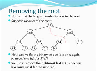
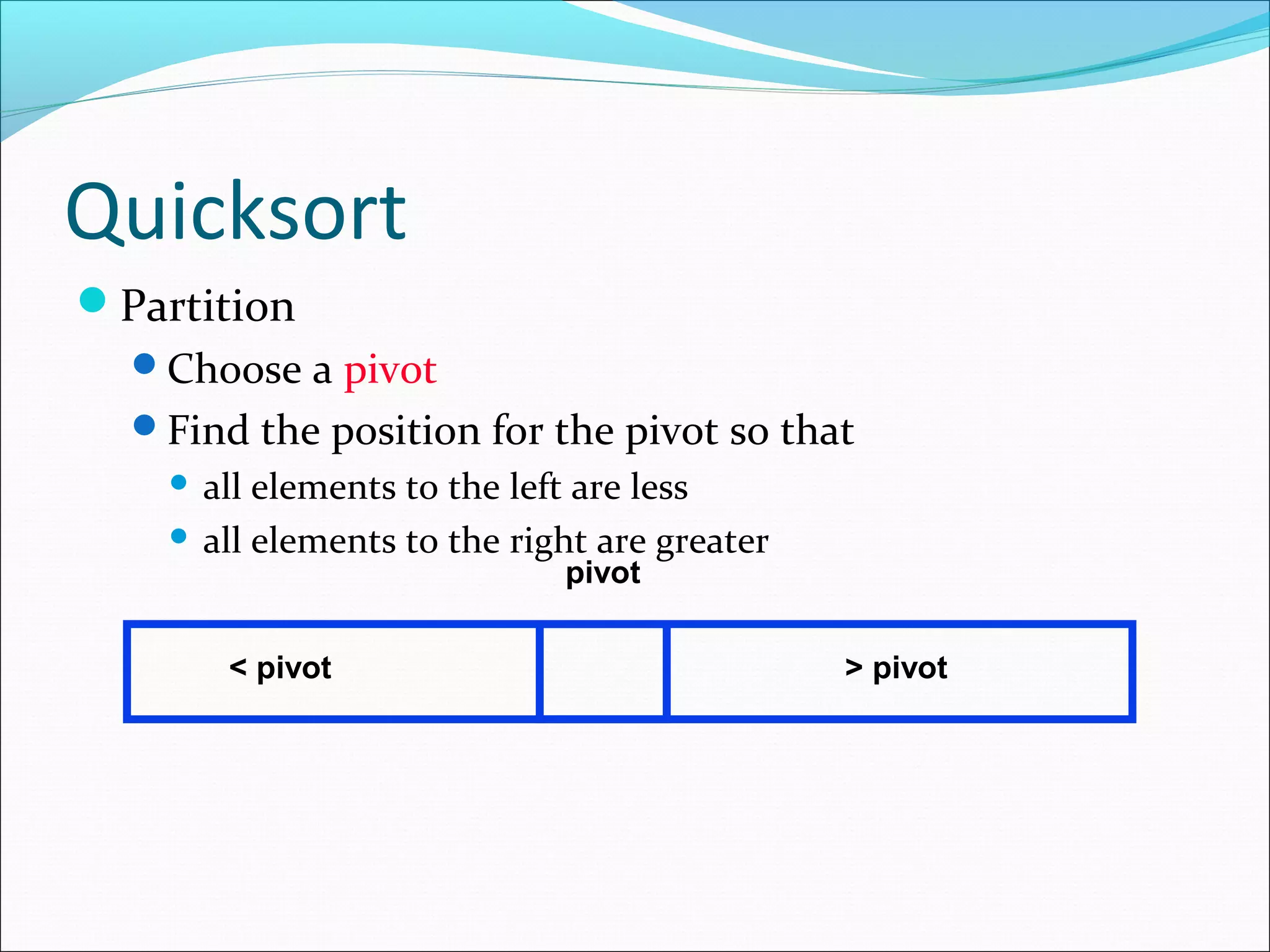
![Quicksort - Partition
int partition( int *a, int low, int high ) {
int left, right;
int pivot_item;
pivot_item = a[low];
pivot = left = low;
right = high;
while ( left < right ) {
/* Move left while item < pivot */
while( a[left] <= pivot_item ) left++;
/* Move right while item > pivot */
while( a[right] >= pivot_item ) right--;
if ( left < right ) SWAP(a,left,right);
}
/* right is final position for the pivot */
a[low] = a[right];
a[right] = pivot_item;
return right;
}](https://image.slidesharecdn.com/sortingalgos-140215040112-phpapp02/85/Sorting-algos-Data-Structures-Algorithums-28-320.jpg)
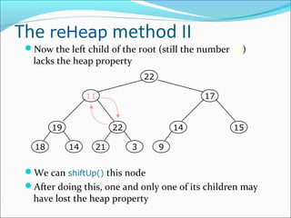
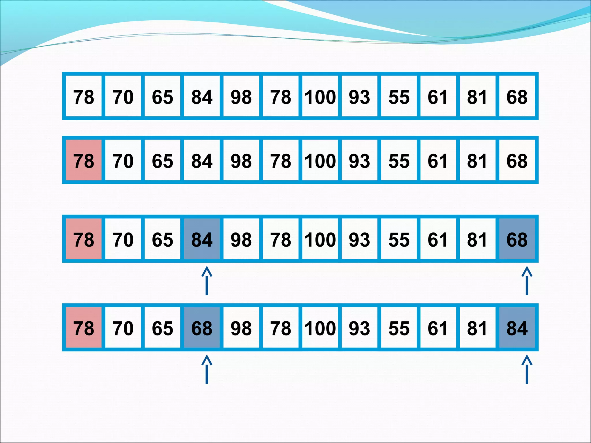
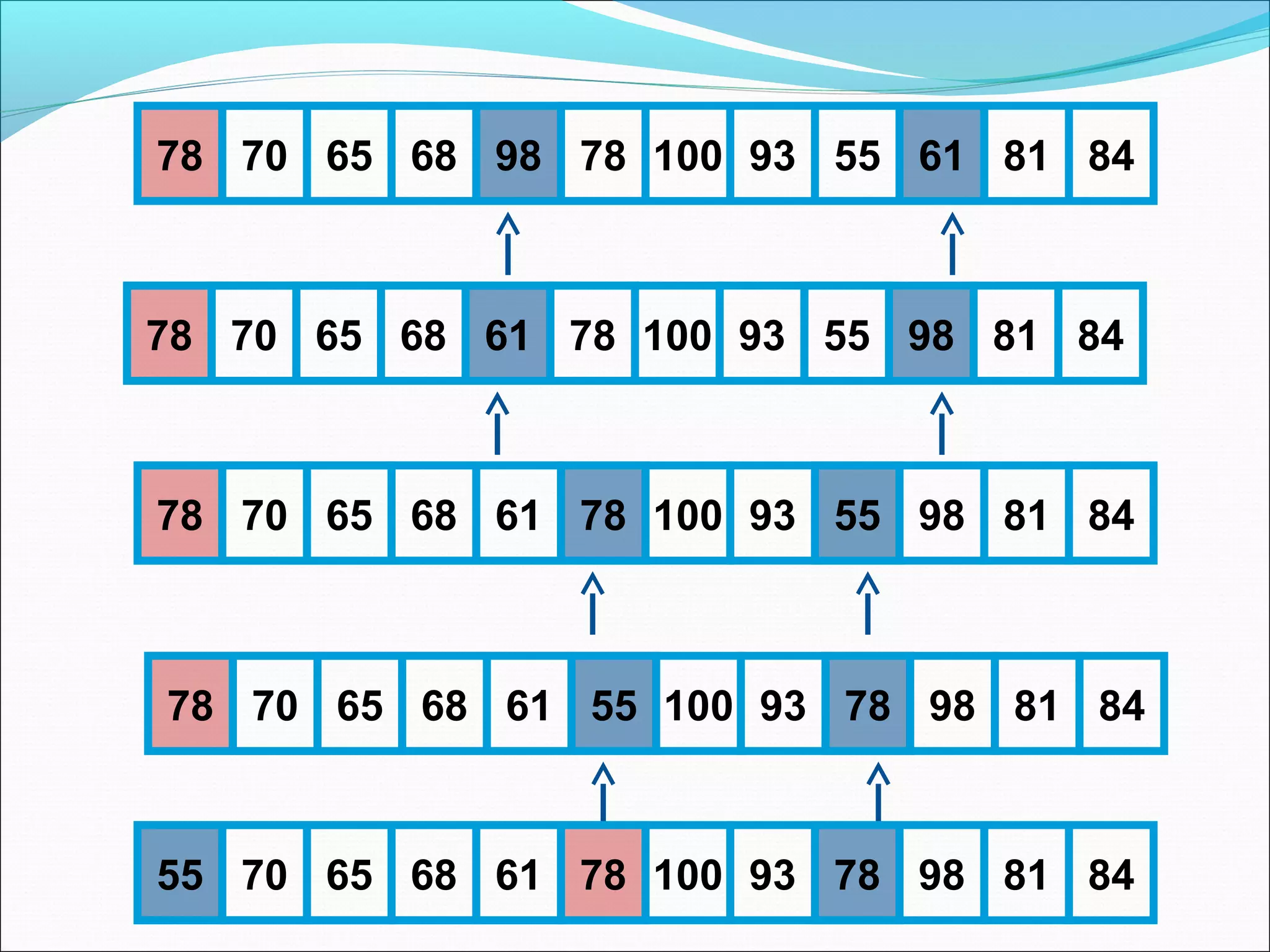
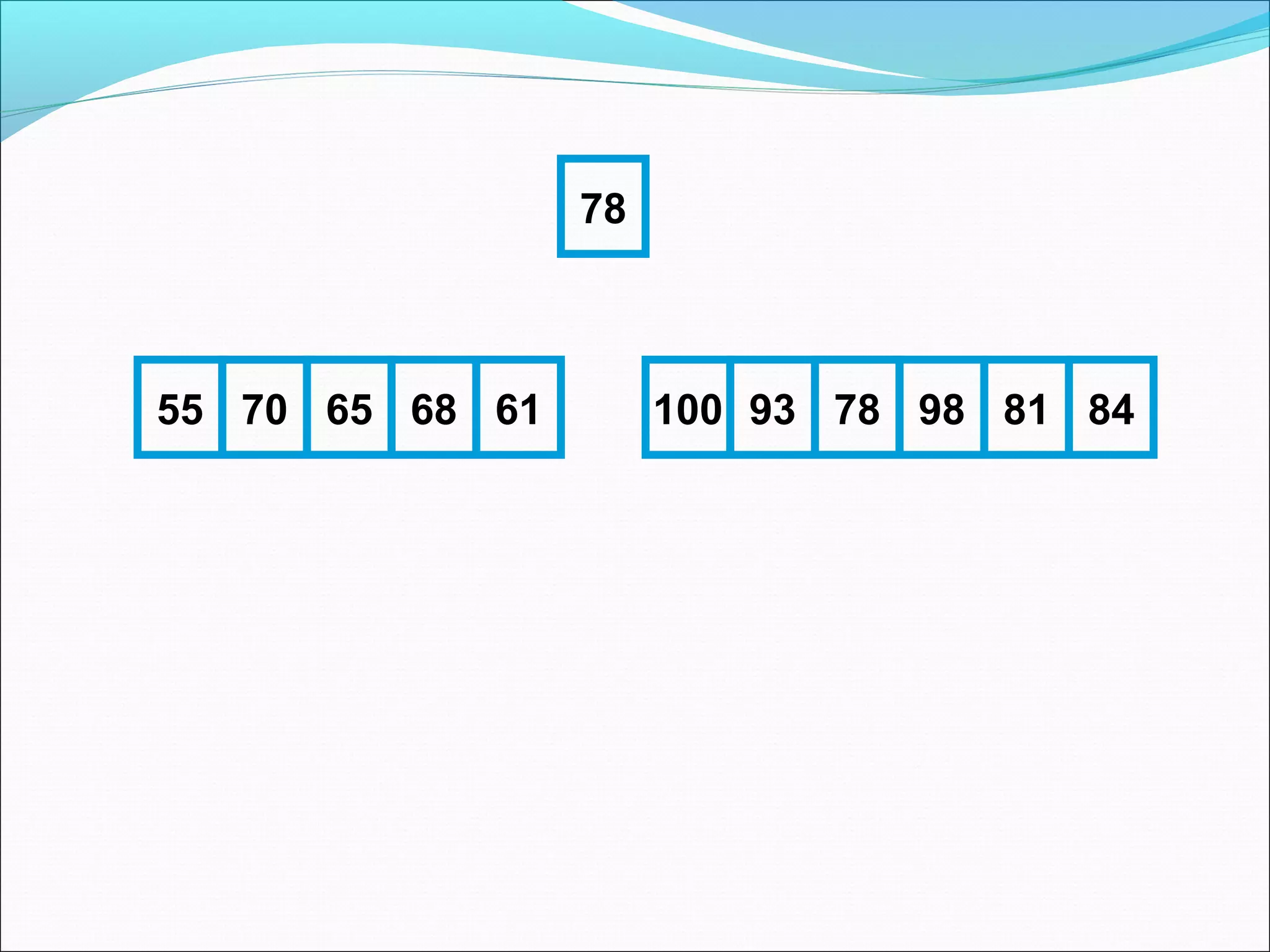
![Quicksort - Partition
This example
uses int’s
to keep things
simple!
int partition( int *a, int low, int high ) {
int left, right;
int pivot_item;
pivot_item = a[low];
pivot = left = low;
right = high;
Any item will do as the pivot,
while ( left < right ) { choose the leftmost one!
/* Move left while item < pivot */
while( a[left] <= pivot_item ) left++;
/* Move right while item > pivot */
while( a[right] >= pivot_item ) right--;
if ( left < right ) SWAP(a,left,right);
}
23 12 15 38 42 18 36 29 27
/* right is final position for the pivot */
a[low] = a[right];
a[right] = pivot_item;
return right;
low
high
}](https://image.slidesharecdn.com/sortingalgos-140215040112-phpapp02/85/Sorting-algos-Data-Structures-Algorithums-29-320.jpg)
![Quicksort - Partition
int partition( int *a, int low, int high ) {
int left, right;
int pivot_item;
pivot_item = a[low];
pivot = left = low;
Set left and right markers
right = high;
while ( left < right ) {
/* Move left while item < pivot */
while( a[left] <= pivot_item ) left++; right
left
/* Move right while item > pivot */
while( a[right] >= pivot_item ) right--;
if (23 12 right 38 SWAP(a,left,right);27
left < 15
) 42 18 36 29
}
/* right is final position for the pivot */
a[low]low a[right];
=
high
pivot: 23
a[right] = pivot_item;
return right;
}](https://image.slidesharecdn.com/sortingalgos-140215040112-phpapp02/85/Sorting-algos-Data-Structures-Algorithums-30-320.jpg)
![Quicksort - Partition
int partition( int *a, int low, int high ) {
int left, right;
int pivot_item;
pivot_item = a[low];
pivot = left = low;
right = high;
Move the markers
until they cross over
while ( left < right ) {
/* Move left while item < pivot */
while( a[left] <= pivot_item ) left++;
/* Move right while item > pivot */
while( a[right] >= pivot_item ) right--;
if ( left < right ) SWAP(a,left,right);
left
}
/* right is final position for the pivot */
a[low] = a[right]; 15 38 42 18 36 29
23 12
a[right] = pivot_item;
return right;
low
pivot: 23
}
right
27
high](https://image.slidesharecdn.com/sortingalgos-140215040112-phpapp02/85/Sorting-algos-Data-Structures-Algorithums-31-320.jpg)
![Quicksort - Partition
int partition( int *a, int low, int high ) {
int left, right;
int pivot_item;
pivot_item = a[low];
pivot = left = low;
right = high;
Move the left pointer while
it points to items <= pivot
while ( left < right ) {
/* Move left while item < pivot */
while( a[left] <= pivot_item ) left++;
/* Move right while item > pivot */
while( a[right] >= pivot_item ) right--;
if ( left < right ) SWAP(a,left,right);
left
right
}
Move right
/* right is final position for the pivot */ similarly
a[low] = a[right];
23 12 15 38 42
a[right] = pivot_item; 18 36 29 27
return right;
}
low
high
pivot: 23](https://image.slidesharecdn.com/sortingalgos-140215040112-phpapp02/85/Sorting-algos-Data-Structures-Algorithums-32-320.jpg)
![Quicksort - Partition
int partition( int *a, int low, int high ) {
int left, right;
int pivot_item;
pivot_item = a[low];
pivot = left = low;
right = high;
Swap the two items
on the wrong side of the pivot
while ( left < right ) {
/* Move left while item < pivot */
while( a[left] <= pivot_item ) left++;
/* Move right while item > pivot */
while( a[right] >= pivot_item ) right--;
if ( left < right ) SWAP(a,left,right);
}
left
right
/* right is final position for the pivot */
a[low] = a[right];
a[right] = pivot_item; 18 36 29 27
23 12 15 38 42
return right;
pivot: 23
}
low
high](https://image.slidesharecdn.com/sortingalgos-140215040112-phpapp02/85/Sorting-algos-Data-Structures-Algorithums-33-320.jpg)
![Quicksort - Partition
int partition( int *a, int low, int high ) {
int left, right;
int pivot_item;
pivot_item = a[low];
pivot = left = low;
right = high;
left and right
have swapped over,
so stop
while ( left < right ) {
/* Move left while item < pivot */
while( a[left] <= pivot_item ) left++;
/* Move right while item > pivot */
while( a[right] >= pivot_item ) right--;
if ( left < right ) SWAP(a,left,right);
}
right
left
/* right is final position for the pivot */
a[low] = a[right];
a[right] = pivot_item; 38 36 29 27
23 12 15 18 42
return right;
}
low
high
pivot: 23](https://image.slidesharecdn.com/sortingalgos-140215040112-phpapp02/85/Sorting-algos-Data-Structures-Algorithums-34-320.jpg)
![Quicksort - Partition
int partition( int *a, int low, int high ) {
int left, right;
int pivot_item;
pivot_item = a[low];
pivot = left = low;
right = high;
right
left
while ( left < right ) {
/* Move left while item < pivot */
23
while( 18 42 38 36 29 27
12 15 a[left] <= pivot_item ) left++;
/* Move right while item > pivot */
while( a[right] >= pivot_item ) right--;
if ( left < right ) SWAP(a,left,right);
low
high
pivot: 23
}
/* right is final position for the pivot */
a[low] = a[right];
Finally, swap the pivot
a[right] = pivot_item;
and right
return right;
}](https://image.slidesharecdn.com/sortingalgos-140215040112-phpapp02/85/Sorting-algos-Data-Structures-Algorithums-35-320.jpg)
![Quicksort - Partition
int partition( int *a, int low, int high ) {
int left, right;
int pivot_item;
pivot_item = a[low];
pivot = left = low;
right = high;
right
while ( left < right ) {
/* Move left while item < pivot */
18
pivot: 23
while( 23 42 38 36 29 27
12 15 a[left] <= pivot_item ) left++;
/* Move right while item > pivot */
while( a[right] >= pivot_item ) right--;
if ( left < right ) SWAP(a,left,right);
low
high
}
/* right is final position for the pivot */
a[low] = a[right];
Return the position
a[right] = pivot_item; of the pivot
return right;
}](https://image.slidesharecdn.com/sortingalgos-140215040112-phpapp02/85/Sorting-algos-Data-Structures-Algorithums-36-320.jpg)


![Static Method mergeSort()
Public static void mergeSort(a, int left, int right)
{
// sort a[left:right]
if (left < right)
{// at least two elements
int mid = (left+right)/2;
//midpoint
mergeSort(a, left, mid);
mergeSort(a, mid + 1, right);
merge(a, b, left, mid, right); //merge from a to b
copy(b, a, left, right); //copy result back to a
}
}](https://image.slidesharecdn.com/sortingalgos-140215040112-phpapp02/75/Sorting-algos-Data-Structures-Algorithums-15-2048.jpg)


![Quicksort - Partition
int partition( int *a, int low, int high ) {
int left, right;
int pivot_item;
pivot_item = a[low];
pivot = left = low;
right = high;
while ( left < right ) {
/* Move left while item < pivot */
while( a[left] <= pivot_item ) left++;
/* Move right while item > pivot */
while( a[right] >= pivot_item ) right--;
if ( left < right ) SWAP(a,left,right);
}
/* right is final position for the pivot */
a[low] = a[right];
a[right] = pivot_item;
return right;
}](https://image.slidesharecdn.com/sortingalgos-140215040112-phpapp02/75/Sorting-algos-Data-Structures-Algorithums-28-2048.jpg)
![Quicksort - Partition
This example
uses int’s
to keep things
simple!
int partition( int *a, int low, int high ) {
int left, right;
int pivot_item;
pivot_item = a[low];
pivot = left = low;
right = high;
Any item will do as the pivot,
while ( left < right ) { choose the leftmost one!
/* Move left while item < pivot */
while( a[left] <= pivot_item ) left++;
/* Move right while item > pivot */
while( a[right] >= pivot_item ) right--;
if ( left < right ) SWAP(a,left,right);
}
23 12 15 38 42 18 36 29 27
/* right is final position for the pivot */
a[low] = a[right];
a[right] = pivot_item;
return right;
low
high
}](https://image.slidesharecdn.com/sortingalgos-140215040112-phpapp02/75/Sorting-algos-Data-Structures-Algorithums-29-2048.jpg)
![Quicksort - Partition
int partition( int *a, int low, int high ) {
int left, right;
int pivot_item;
pivot_item = a[low];
pivot = left = low;
Set left and right markers
right = high;
while ( left < right ) {
/* Move left while item < pivot */
while( a[left] <= pivot_item ) left++; right
left
/* Move right while item > pivot */
while( a[right] >= pivot_item ) right--;
if (23 12 right 38 SWAP(a,left,right);27
left < 15
) 42 18 36 29
}
/* right is final position for the pivot */
a[low]low a[right];
=
high
pivot: 23
a[right] = pivot_item;
return right;
}](https://image.slidesharecdn.com/sortingalgos-140215040112-phpapp02/75/Sorting-algos-Data-Structures-Algorithums-30-2048.jpg)
![Quicksort - Partition
int partition( int *a, int low, int high ) {
int left, right;
int pivot_item;
pivot_item = a[low];
pivot = left = low;
right = high;
Move the markers
until they cross over
while ( left < right ) {
/* Move left while item < pivot */
while( a[left] <= pivot_item ) left++;
/* Move right while item > pivot */
while( a[right] >= pivot_item ) right--;
if ( left < right ) SWAP(a,left,right);
left
}
/* right is final position for the pivot */
a[low] = a[right]; 15 38 42 18 36 29
23 12
a[right] = pivot_item;
return right;
low
pivot: 23
}
right
27
high](https://image.slidesharecdn.com/sortingalgos-140215040112-phpapp02/75/Sorting-algos-Data-Structures-Algorithums-31-2048.jpg)
![Quicksort - Partition
int partition( int *a, int low, int high ) {
int left, right;
int pivot_item;
pivot_item = a[low];
pivot = left = low;
right = high;
Move the left pointer while
it points to items <= pivot
while ( left < right ) {
/* Move left while item < pivot */
while( a[left] <= pivot_item ) left++;
/* Move right while item > pivot */
while( a[right] >= pivot_item ) right--;
if ( left < right ) SWAP(a,left,right);
left
right
}
Move right
/* right is final position for the pivot */ similarly
a[low] = a[right];
23 12 15 38 42
a[right] = pivot_item; 18 36 29 27
return right;
}
low
high
pivot: 23](https://image.slidesharecdn.com/sortingalgos-140215040112-phpapp02/75/Sorting-algos-Data-Structures-Algorithums-32-2048.jpg)
![Quicksort - Partition
int partition( int *a, int low, int high ) {
int left, right;
int pivot_item;
pivot_item = a[low];
pivot = left = low;
right = high;
Swap the two items
on the wrong side of the pivot
while ( left < right ) {
/* Move left while item < pivot */
while( a[left] <= pivot_item ) left++;
/* Move right while item > pivot */
while( a[right] >= pivot_item ) right--;
if ( left < right ) SWAP(a,left,right);
}
left
right
/* right is final position for the pivot */
a[low] = a[right];
a[right] = pivot_item; 18 36 29 27
23 12 15 38 42
return right;
pivot: 23
}
low
high](https://image.slidesharecdn.com/sortingalgos-140215040112-phpapp02/75/Sorting-algos-Data-Structures-Algorithums-33-2048.jpg)
![Quicksort - Partition
int partition( int *a, int low, int high ) {
int left, right;
int pivot_item;
pivot_item = a[low];
pivot = left = low;
right = high;
left and right
have swapped over,
so stop
while ( left < right ) {
/* Move left while item < pivot */
while( a[left] <= pivot_item ) left++;
/* Move right while item > pivot */
while( a[right] >= pivot_item ) right--;
if ( left < right ) SWAP(a,left,right);
}
right
left
/* right is final position for the pivot */
a[low] = a[right];
a[right] = pivot_item; 38 36 29 27
23 12 15 18 42
return right;
}
low
high
pivot: 23](https://image.slidesharecdn.com/sortingalgos-140215040112-phpapp02/75/Sorting-algos-Data-Structures-Algorithums-34-2048.jpg)
![Quicksort - Partition
int partition( int *a, int low, int high ) {
int left, right;
int pivot_item;
pivot_item = a[low];
pivot = left = low;
right = high;
right
left
while ( left < right ) {
/* Move left while item < pivot */
23
while( 18 42 38 36 29 27
12 15 a[left] <= pivot_item ) left++;
/* Move right while item > pivot */
while( a[right] >= pivot_item ) right--;
if ( left < right ) SWAP(a,left,right);
low
high
pivot: 23
}
/* right is final position for the pivot */
a[low] = a[right];
Finally, swap the pivot
a[right] = pivot_item;
and right
return right;
}](https://image.slidesharecdn.com/sortingalgos-140215040112-phpapp02/75/Sorting-algos-Data-Structures-Algorithums-35-2048.jpg)
![Quicksort - Partition
int partition( int *a, int low, int high ) {
int left, right;
int pivot_item;
pivot_item = a[low];
pivot = left = low;
right = high;
right
while ( left < right ) {
/* Move left while item < pivot */
18
pivot: 23
while( 23 42 38 36 29 27
12 15 a[left] <= pivot_item ) left++;
/* Move right while item > pivot */
while( a[right] >= pivot_item ) right--;
if ( left < right ) SWAP(a,left,right);
low
high
}
/* right is final position for the pivot */
a[low] = a[right];
Return the position
a[right] = pivot_item; of the pivot
return right;
}](https://image.slidesharecdn.com/sortingalgos-140215040112-phpapp02/75/Sorting-algos-Data-Structures-Algorithums-36-2048.jpg)


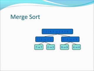
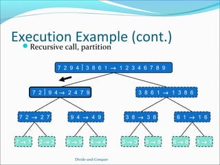
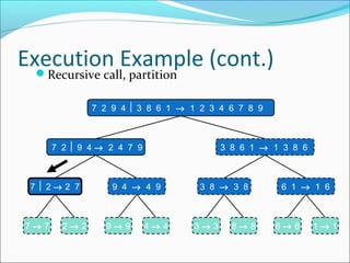
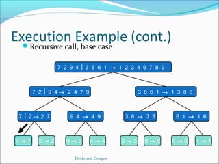
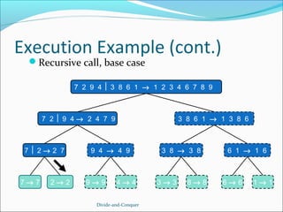
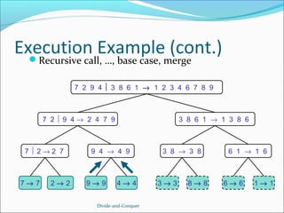
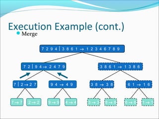
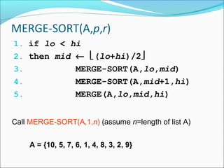
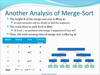
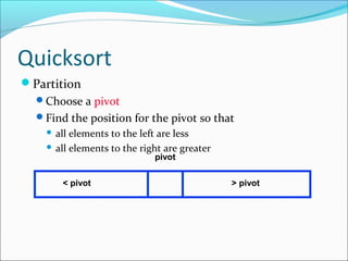
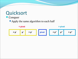
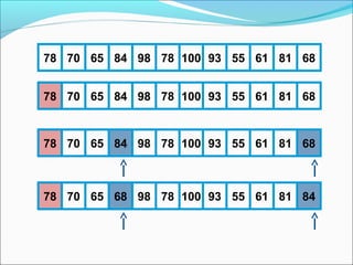
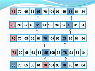
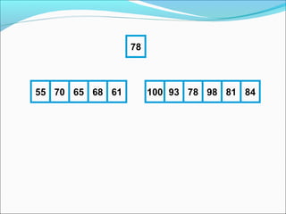
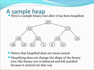
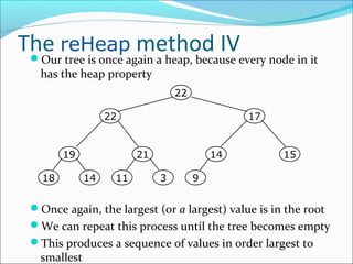
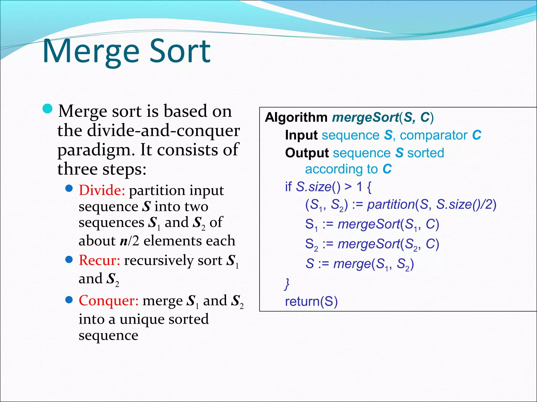
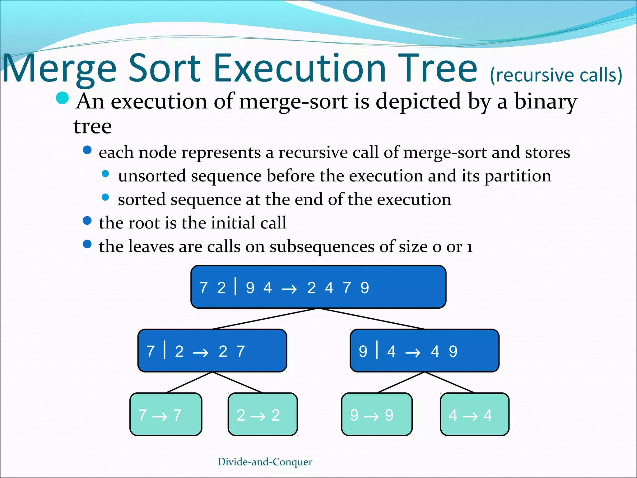
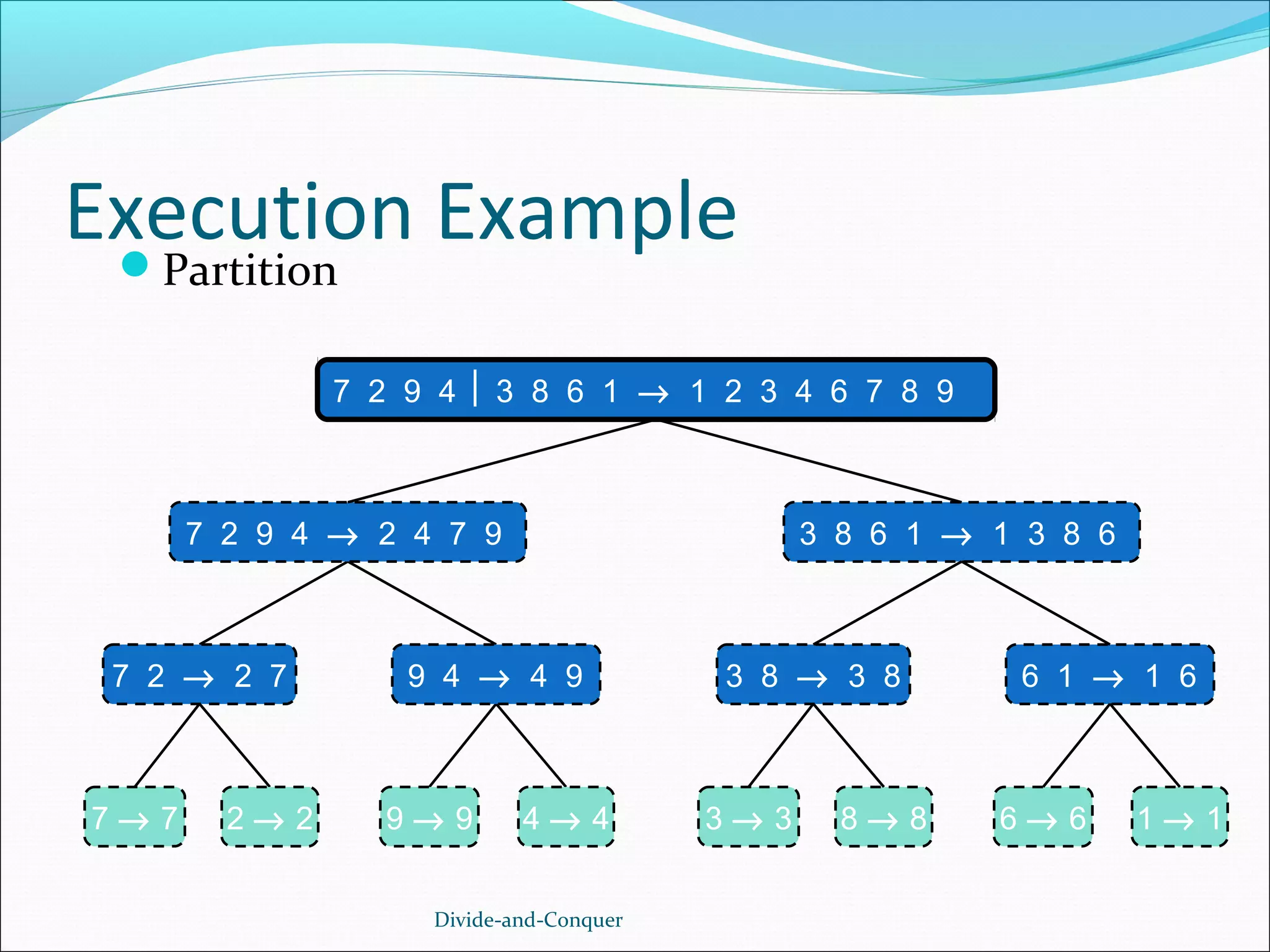
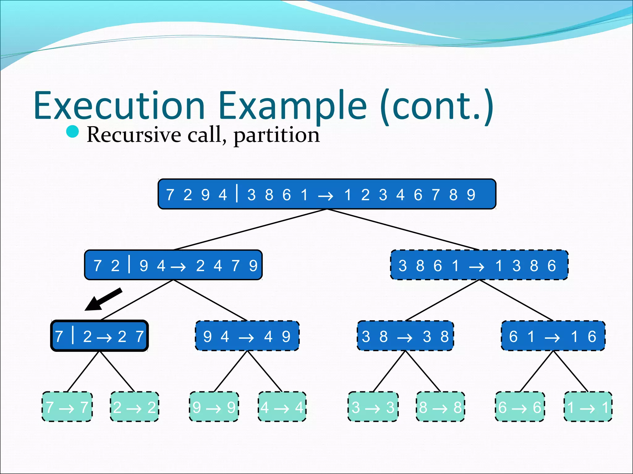
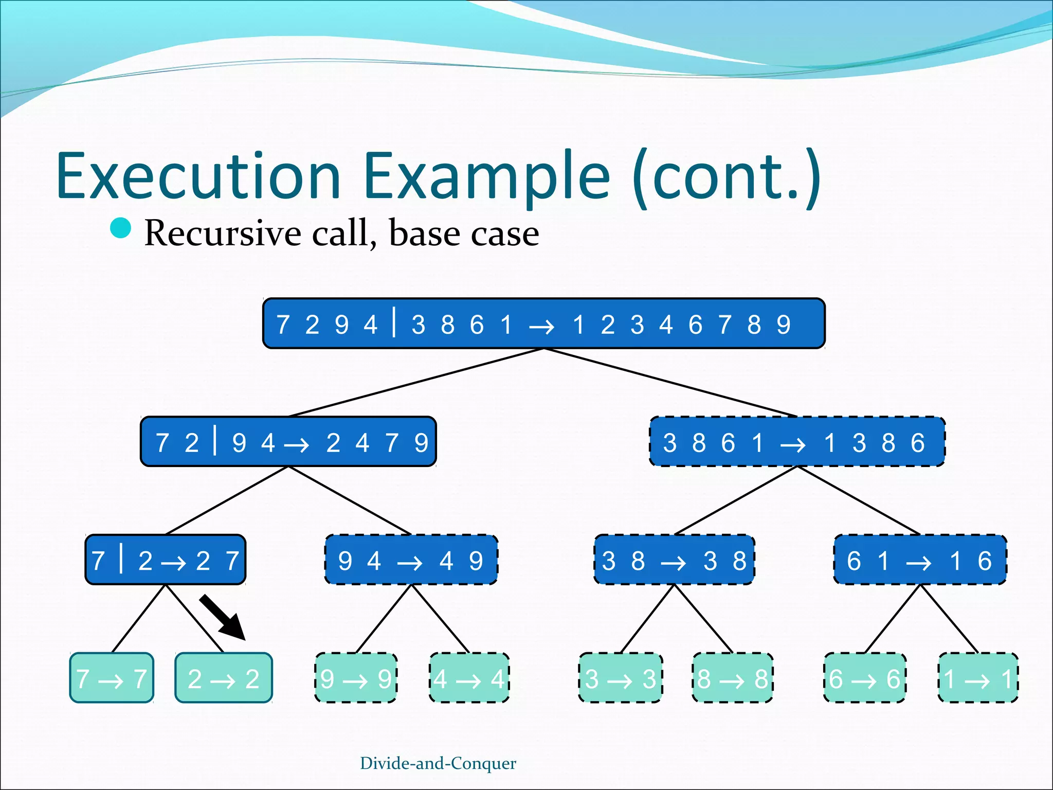
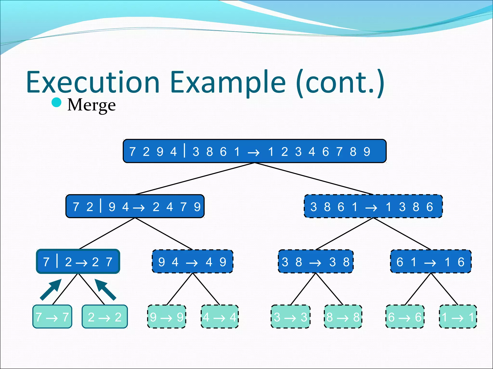
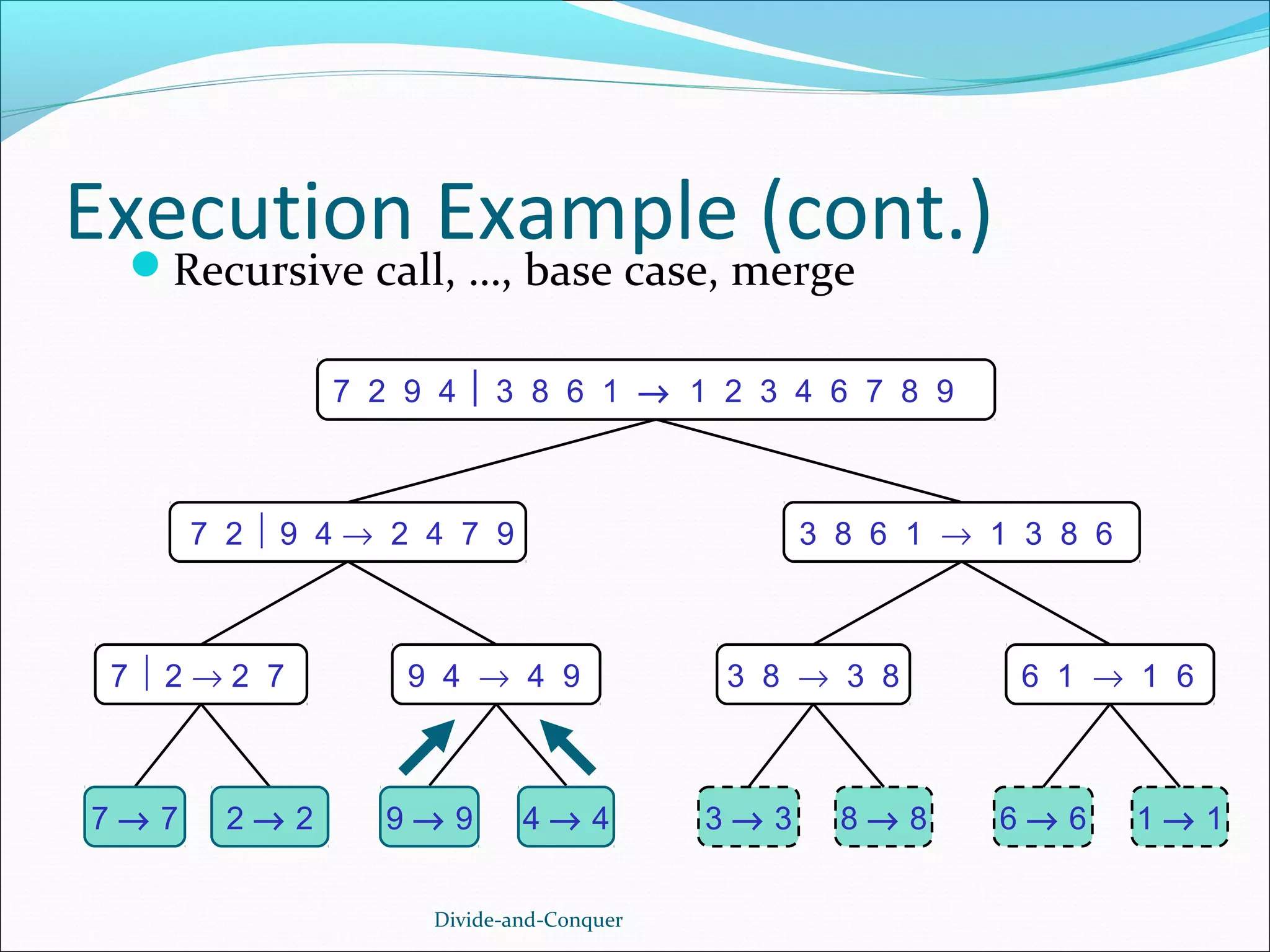
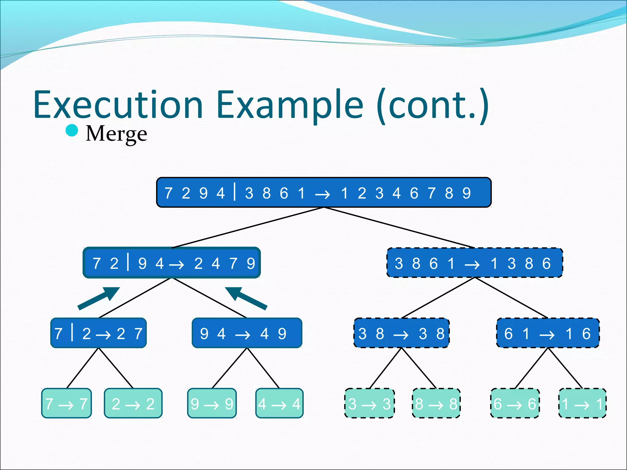
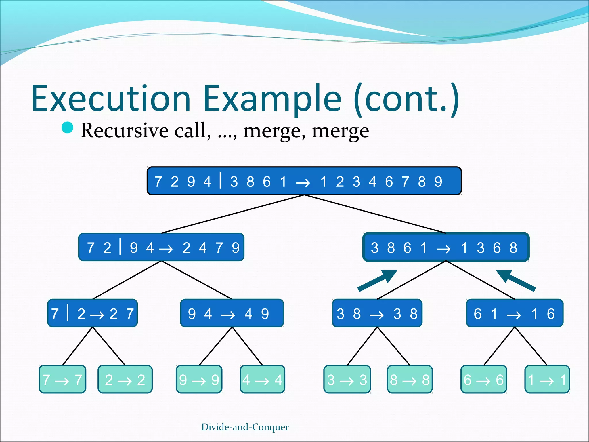
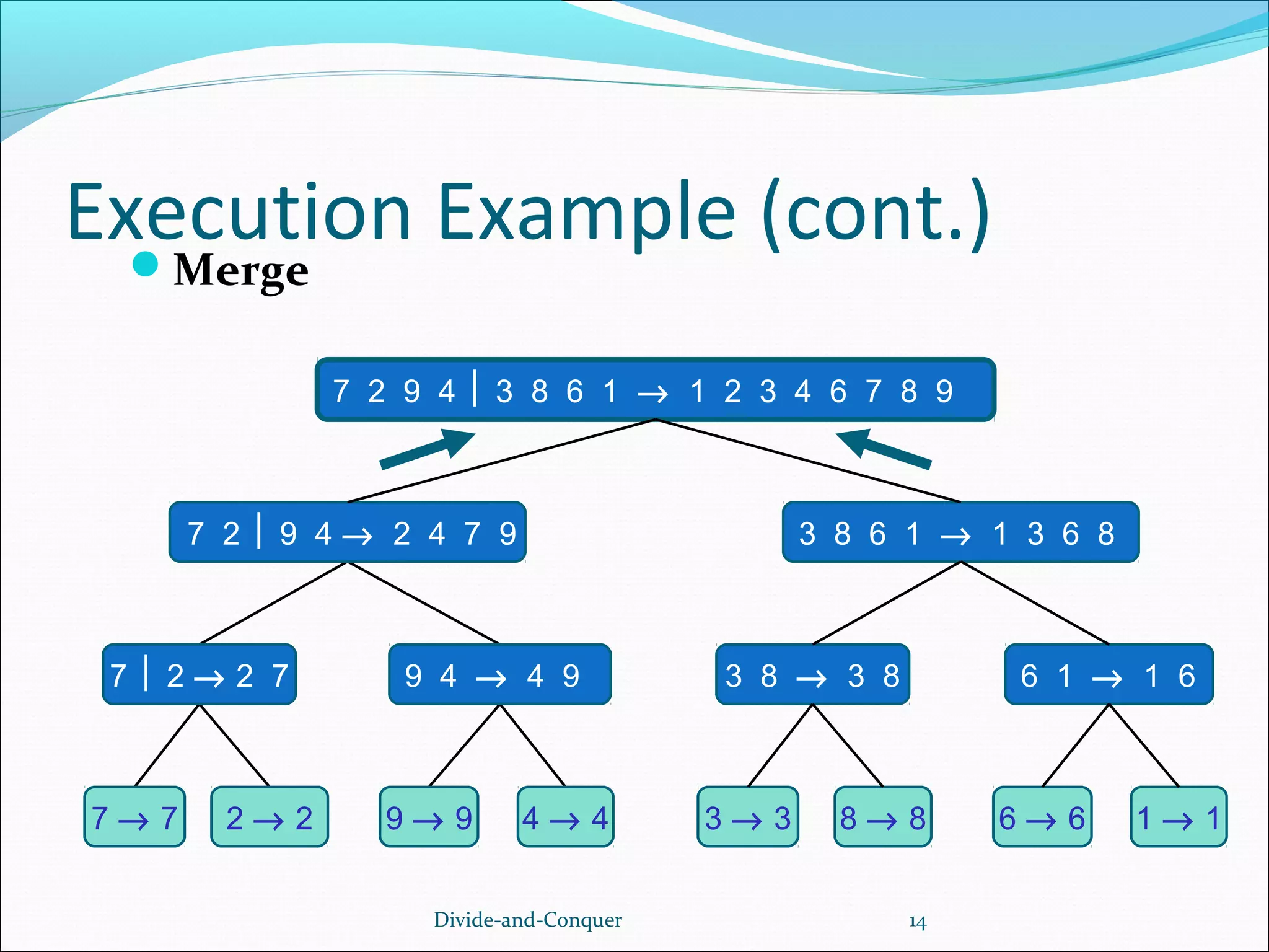
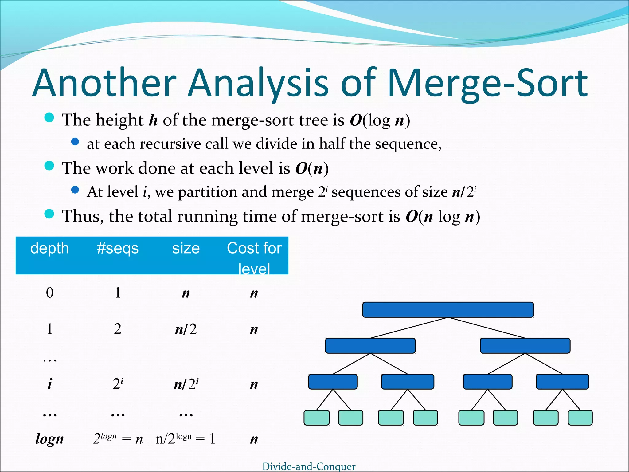
The document describes the merge sort algorithm. Merge sort is a sorting algorithm that works by dividing an unsorted list into halves, recursively sorting each half, and then merging the sorted halves into one sorted list. It has the following steps: 1. Divide: Partition the input list into equal halves. 2. Conquer: Recursively sort each half by repeating steps 1 and 2. 3. Combine: Merge the sorted halves into one sorted output list. The algorithm has a runtime of O(n log n), making it an efficient sorting algorithm for large data sets. An example execution is shown step-by-step to demonstrate how merge sort partitions, recursively sorts, and merges sublists to produce


![UNIT V Searching Sorting Hashing Techniques [Autosaved].pptx](https://cdn.slidesharecdn.com/ss_thumbnails/unitvsearchingsortinghashingtechniquesautosaved-241126054304-95a69c51-thumbnail.jpg?width=600ounds&width=560&fit=bounds)


![UNIT V Searching Sorting Hashing Techniques [Autosaved].pptx](https://cdn.slidesharecdn.com/ss_thumbnails/unitvsearchingsortinghashingtechniquesautosaved-241014040608-74caa0f6-thumbnail.jpg?width=600ounds&width=560&fit=bounds)


