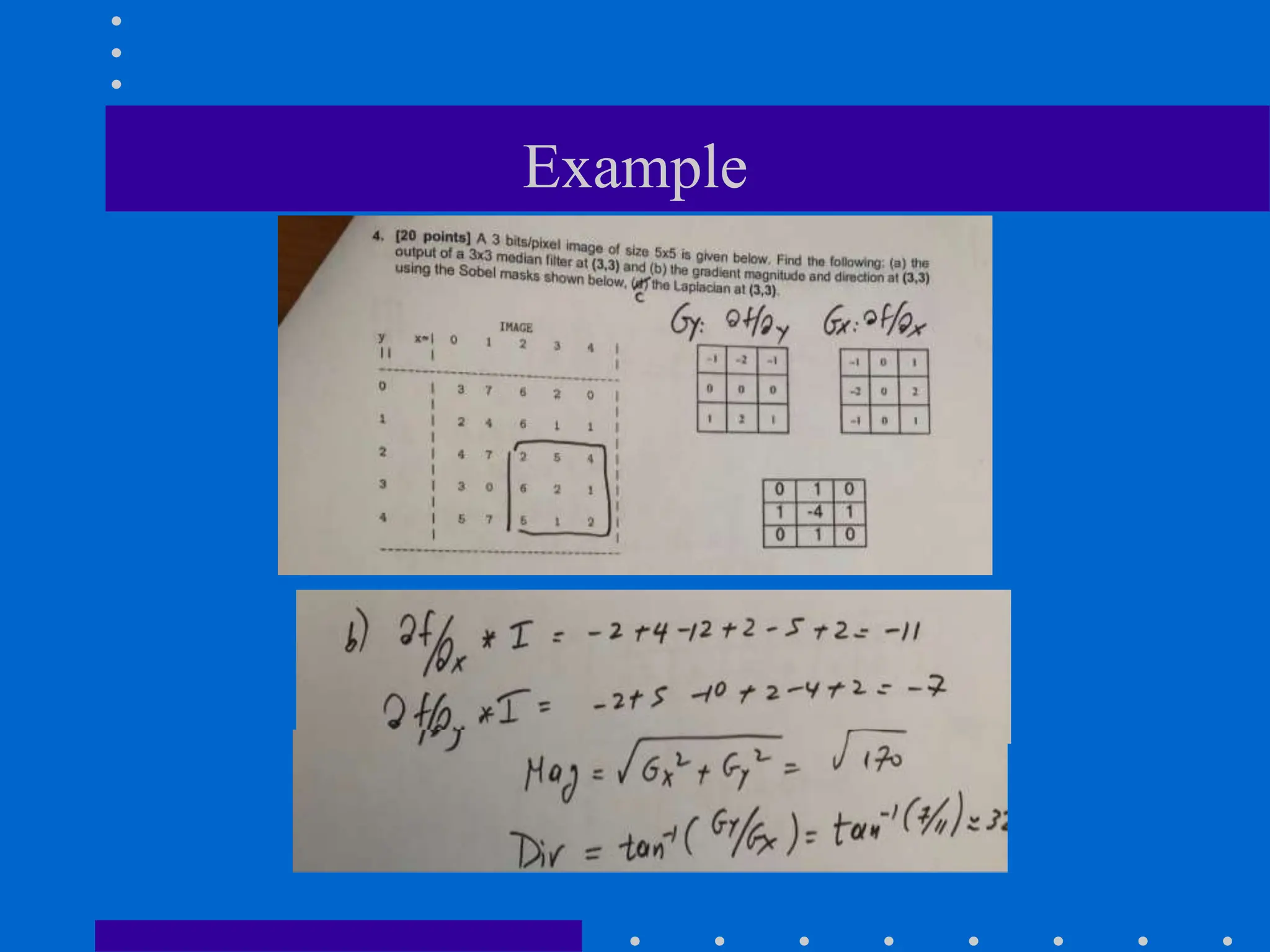
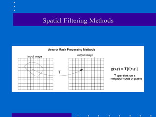
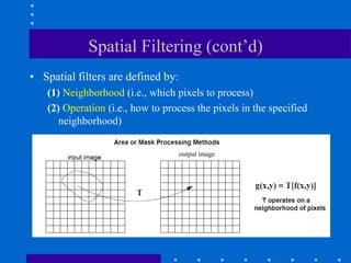
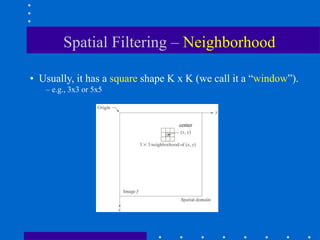
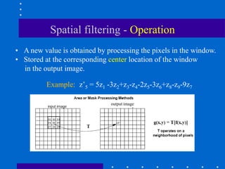
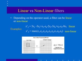
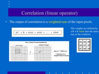
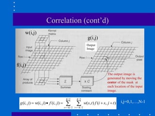
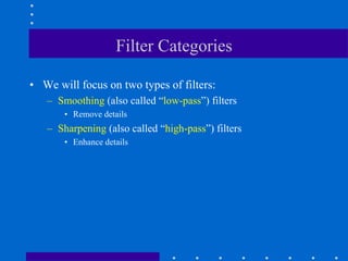
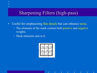
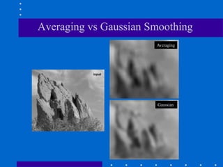
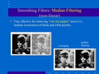
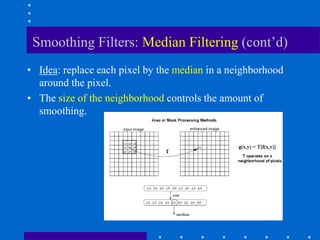
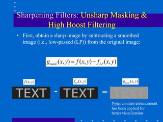
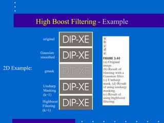
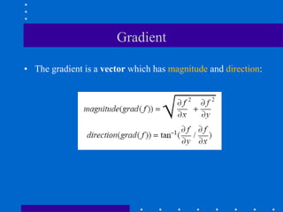
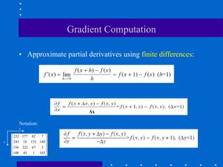
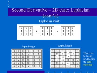
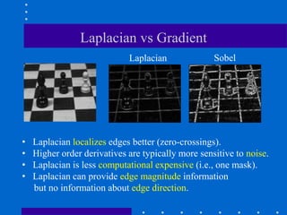
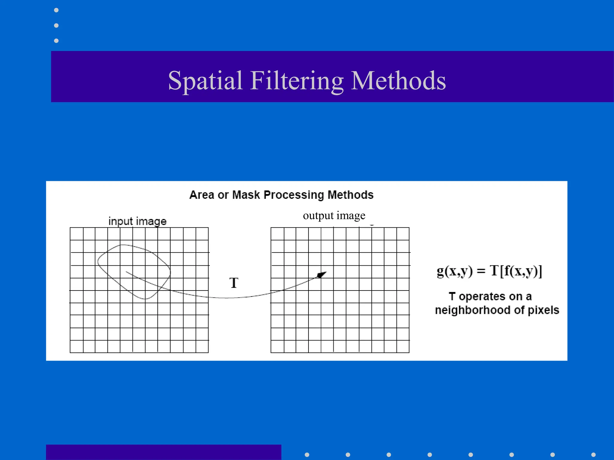
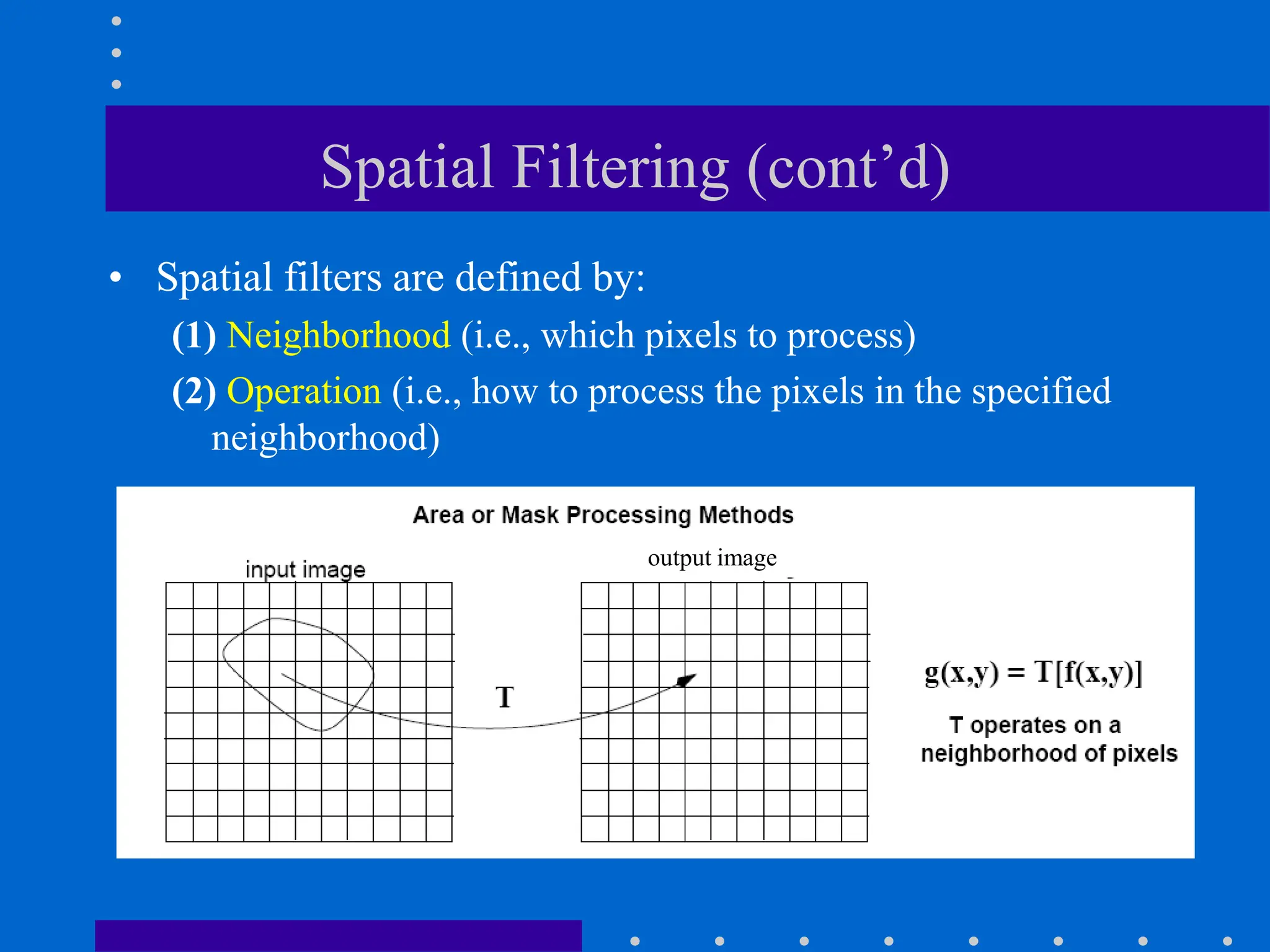
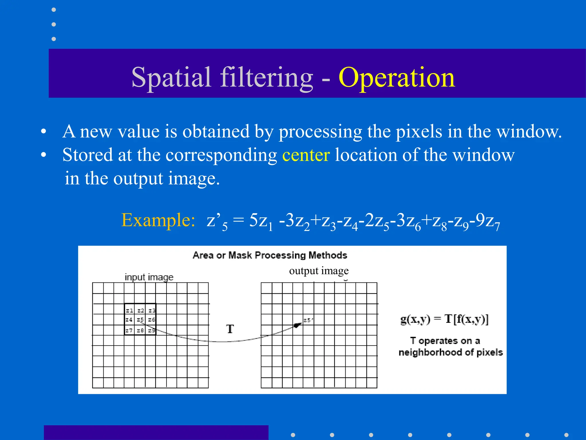
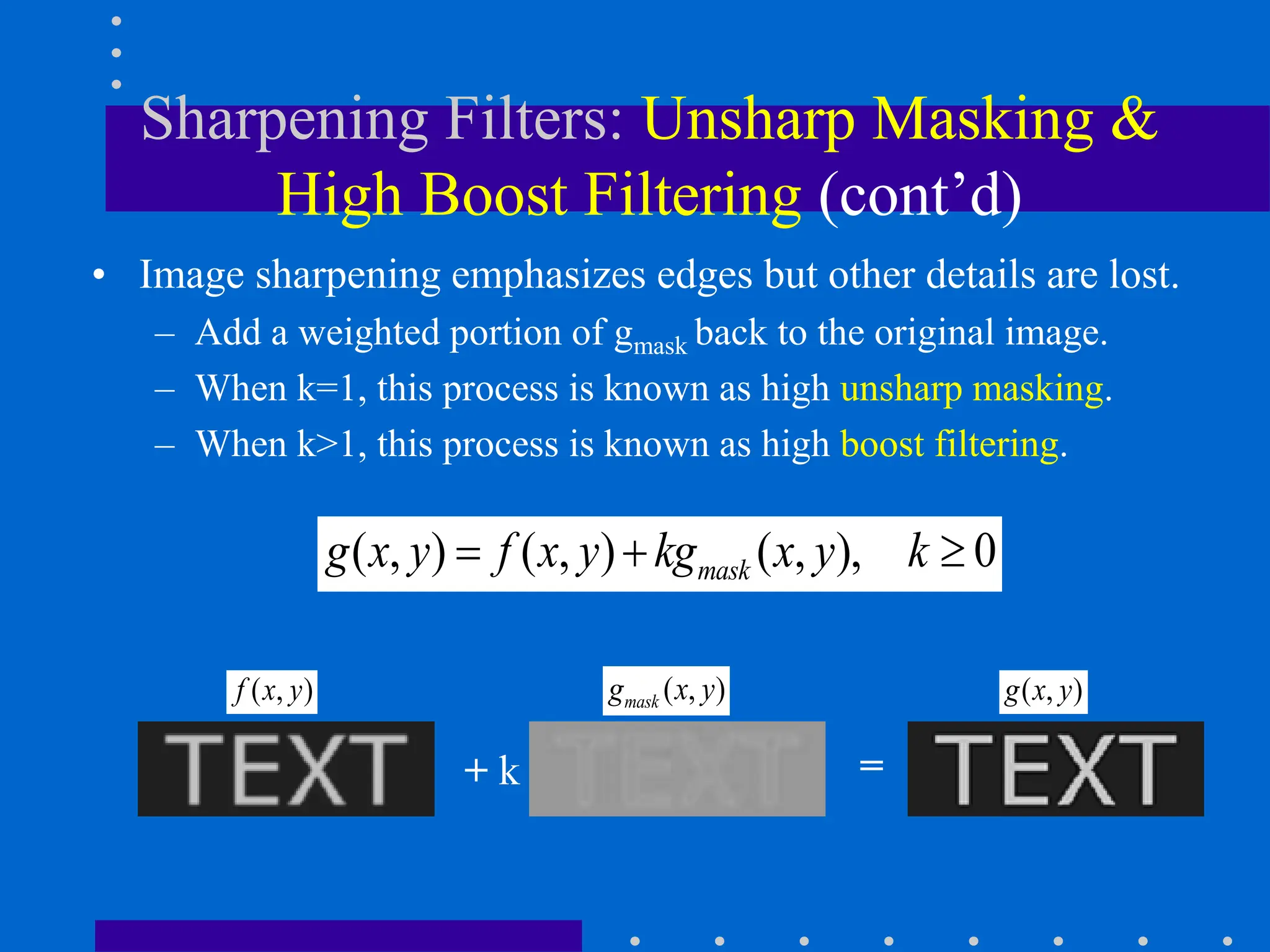
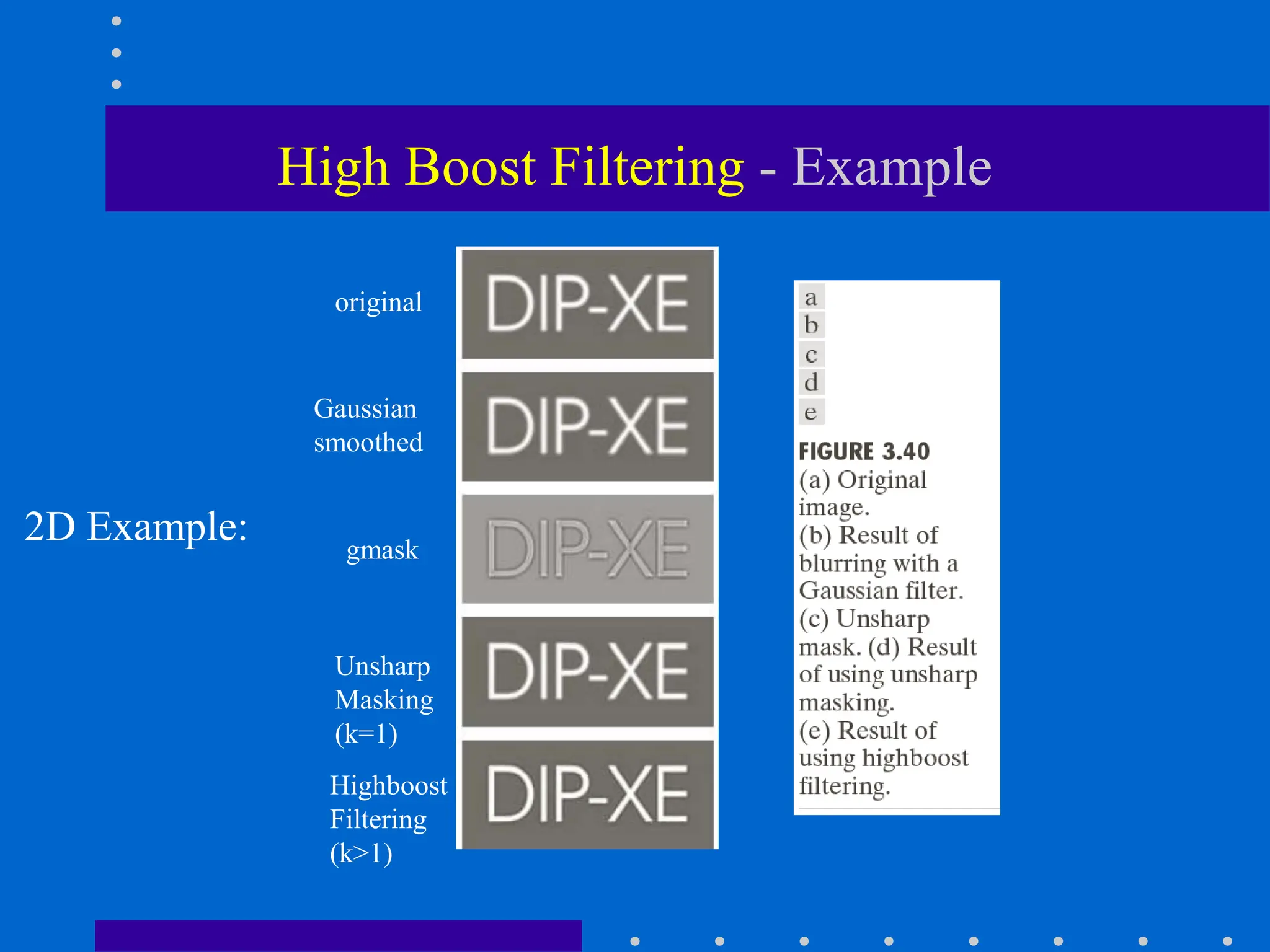
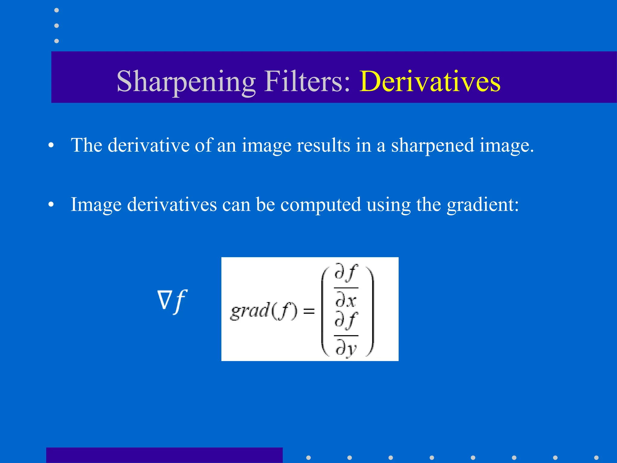
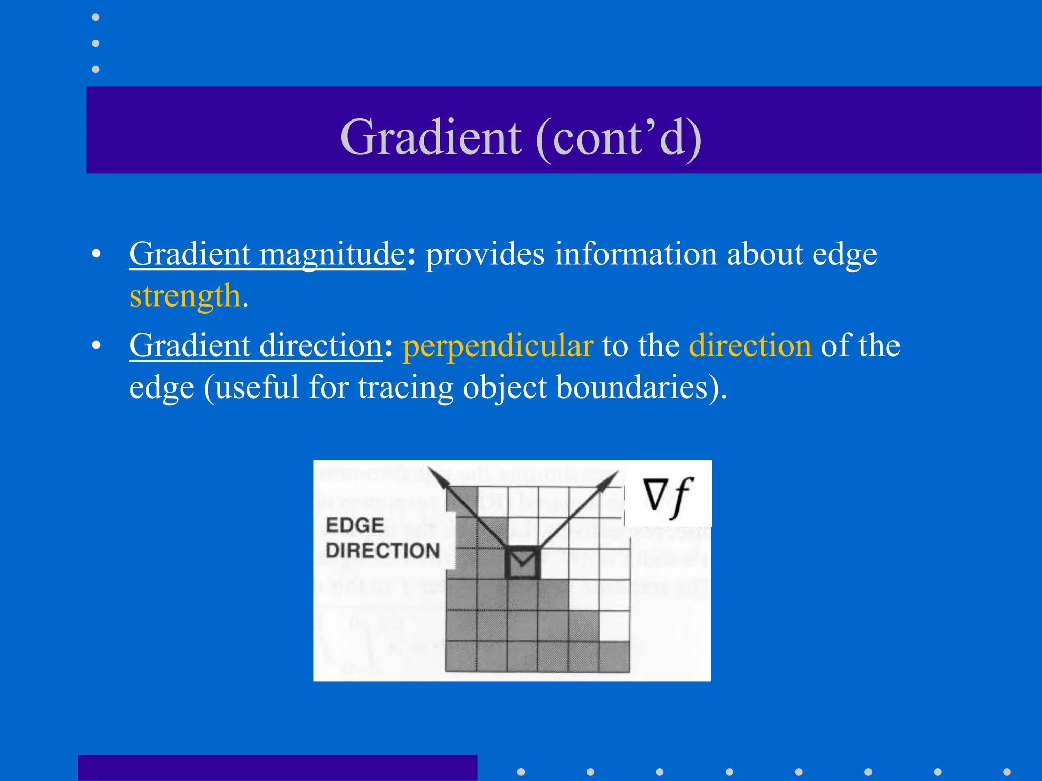
KEMBAR78
Spatial Filtering in intro image processingr | PPT
Spatial Filtering
CS474/674 - Prof. Bebis
Sections 3.4, 3.5, 3.6, 3.7, 3.8
Spatial Filtering Methods
output image
Spatial Filtering (cont’d)
• Spatial filters are defined by:
(1) Neighborhood (i.e., which pixels to process)
(2) Operation (i.e., how to process the pixels in the specified
neighborhood)
output image
Spatial Filtering – Neighborhood
• Usually, it has a square shape K x K (we call it a “window”).
– e.g., 3x3 or 5x5
center
Spatial filtering - Operation
output image
• A new value is obtained by processing the pixels in the window.
• Stored at the corresponding center location of the window
in the output image.
z’5 = 5z1 -3z2+z3-z4-2z5-3z6+z8-z9-9z7
Example:
Linear vs Non-Linear filters
• Depending on the operator used, a filter can be linear
or non-linear
output image
z’5 = 5z1 -3z2+z3-z4-2z5-3z6+z8-z9-9z7
Examples:
z’5 = max(z1,z2,z3,z4,z5,z6,z7,z8,z9)
linear
non-linear
Linear Operators
• Two common linear operators are:
– Correlation
– Convolution
• The output is a linear combination of the inputs.
Correlation (linear operator)
output image
• The output of correlation is a weighted sum of the input pixels.
The weights are defined by
a K x K mask (has the same
size as the window):
Correlation (cont’d)
Output
Image
w(i,j)
f(i,j)
/2 /2
/2 /2
( , ) ( , ) ( , ) ( , ) ( , )
K K
s K t K
g i j w i j f i j w s t f i s j t
 
    
 
g(i,j)
The output image is
generated by moving the
center of the mask at
each location of the input
image.
i,j=0,1,…,N-1
Handling Locations Close to Boundaries
Usually, we pad with zeroes
Alternatively, skip the first/last few rows/columns
0 0 0 ……………………….0
0
0
0
……………………….0
Correlation (cont’d)
Often used in applications where
we need to measure the similarity
between an image and a pattern
(e.g., template matching).
Simple template matching
does not work in most
practical cases.
Convolution (linear operator)
• Similar to correlation except that the mask is first flipped
both horizontally and vertically.
• Note: if w(i, j) is symmetric (i.e., w(i, j)=w(-i,-j)), then
convolution is equivalent to correlation!
/2 /2
/2 /2
( , ) ( , ) ( , ) ( , ) ( , )
K K
s K t K
g i j w i j f i j w s t f i s j t
 
    
 
i,j=0,1,…,N-1
Example
Correlation:
Convolution:
Filter Categories
• We will focus on two types of filters:
– Smoothing (also called “low-pass”) filters
• Remove details
– Sharpening (also called “high-pass”) filters
• Enhance details
Smoothing Filters (low-pass)
• Useful for reducing noise and removing small details.
– The elements of the mask must be positive.
– Mask elements sum to 1 assuming normalized weights (i.e.,
divide each weight by the sum of weights).
Smoothing filters – Example
smoothed image
input image
Sharpening Filters (high-pass)
• Useful for emphasizing fine details but can enhance noise.
– The elements of the mask contain both positive and negative
weights.
– Mask elements sum to 0.
Sharpening Filters - Example
• e.g., emphasize edges in an image
Sharpening Filters - Example
sharpened image
input image
Note: for better visualization, the
original image is typically added to
the sharpened image.
Common Smoothing Filters
• Averaging (linear)
• Gaussian (linear)
• Median filtering (non-linear)
Smoothing Filters: Averaging
The mask weights are all equal to 1
Smoothing Filters: Averaging (cont’d)
• Mask size determines degree of smoothing (i.e., loss of detail).
3x3 5x5 7x7
15x15 25x25
original
Smoothing Filters: Averaging (cont’d)
15 x 15 averaging After image thresholding
Example: extract largest, brightest objects
Smoothing filters: Gaussian
• The mask weights are the sampled values of a 2D Gaussian:
Smoothing filters: Gaussian (cont’d)
• Mask size depends on σ, e.g., it is usually chosen as
follows:
Smoothing filters: Gaussian (cont’d)
• In this case, σ controls the amount of smoothing
(since mask size depends on it)
σ = 3
σ = 1.4
Smoothing filters: Gaussian (cont’d)
Example
Averaging vs Gaussian Smoothing
Averaging
Gaussian
Smoothing Filters: Median Filtering
(non-linear)
• Very effective for removing “salt and pepper” noise (i.e.,
random occurrences of black and white pixels).
averaging
median
filtering
Smoothing Filters: Median Filtering (cont’d)
• Idea: replace each pixel by the median in a neighborhood
around the pixel.
• The size of the neighborhood controls the amount of
smoothing.
Sharpening Filters
• Common sharpening filters
– Unsharp masking
– High Boost filtering
– Gradient (1st derivative)
– Laplacian (2nd derivative)
Sharpening Filters: Unsharp Masking &
High Boost Filtering
• First, obtain a sharp image by subtracting a smoothed
image (i.e., low-passed (LP)) from the original image:
- =
Note: contrast enhancement
has been applied for
better visualization
( , ) ( , ) ( , )
mask LP
g x y f x y f x y
 
( , )
mask
g x y
( , )
LP
f x y
( , )
f x y
Sharpening Filters: Unsharp Masking &
High Boost Filtering (cont’d)
• Image sharpening emphasizes edges but other details are lost.
– Add a weighted portion of gmask back to the original image.
– When k=1, this process is known as high unsharp masking.
– When k>1, this process is known as high boost filtering.
+ k =
( , ) ( , ) ( , ), 0
mask
g x y f x y kg x y k
  
( , )
f x y ( , )
mask
g x y ( , )
g x y
High Boost Filtering - Example
original
Gaussian
smoothed
gmask
Unsharp
Masking
(k=1)
Highboost
Filtering
(k>1)
2D Example:
Sharpening Filters: Derivatives
• The derivative of an image results in a sharpened image.
• Image derivatives can be computed using the gradient:
Gradient
• The gradient is a vector which has magnitude and direction:
Gradient (cont’d)
• Gradient magnitude: provides information about edge
strength.
• Gradient direction: perpendicular to the direction of the
edge (useful for tracing object boundaries).
Gradient Computation
• Approximate partial derivatives using finite differences:
Δx
232 177 82 7
241 18 152 140
156 221 67 3
100 45 1 103
 
 
 
 
 
 
x
y
Notation:
Gradient Computation (cont’d)
sensitive to vertical edges
sensitive to horizontal edges
y2=y3+Dy, y3=y, x3=x, Dy=1
Example: visualize partial derivatives
f
x


f
y


• Image derivatives can be visualized as an image
by mapping the values to [0, 255]
Implement Gradient Using Masks
• We can implement and using masks:
(x+1/2,y)
(x,y+1/2)
*
*
good approximation
at (x+1/2,y)
good approximation
at (x,y+1/2)
Derivatives are not
computed at the same
location!
Implement Gradient Using Masks (cont’d)
• A different approximation of the gradient:
• We can implement and using the following masks:
*
(x+1/2,y+1/2)
good approximation
Derivatives are
computed at the
same location!
Implement Gradient Using Masks (cont’d)
• Other approximations
Sobel
Prewitt
Example: Visualize Gradient Magnitude
f
y


f
x


Gradient Magnitude
(isotropic, i.e., detects
edges in all directions)
• The gradient magnitude can be visualized
as an image by mapping the values to [0, 255]
Second Derivative – 1D case
( ) ( 1) ( )
( ) ( 1) ( ) ( 1) ( 1) 2 ( )
f x f x f x
f x f x f x f x f x f x
   
  
       
Second Derivative – 1D case (cont’d)
• Often, points that lie on an edge
can be detected by:
(1) Local maxima or
minima of the first derivative.
(2) Zero-crossings
of the second derivative (i.e., where
the second derivative changes sign). 2nd derivative
1st derivative
Second Derivative – 1D case (cont’d)
Example:
Second Derivative – 2D case: Laplacian
The Laplacian is defined as:
(dot product)
Approximate
2nd partial
derivatives:
Second Derivative – 2D case: Laplacian
(cont’d)
Laplacian Mask
Edges can
be found
by detecting
the zero-
crossings
input image output image
5
5
5
5 5
-5 -5
-10
-10
-10
10
Second Derivative – 2D case: Laplacian
(cont’d)
• Other realizations of the Laplacian mask found in practice.
Visualize the results of the Laplacian
• Add the results of the Laplacian to the original
image for better visualization
2
2
2
( , ) ( , ) ( , )
where,
( , ) is input image,
( , ) is sharpenend images,
-1 if ( , ) has a negative center value
and 1 if ( , ) has a positive center value.
g x y f x y c f x y
f x y
g x y
c f x y
c f x y
 
  
 
 
 
Visualize the results of the Laplacian
(cont’d)
no normalization,
negative values
clipped to zero
blurred image
scaled to [0, 255]
Example:
Laplacian vs Gradient
Laplacian Sobel
• Laplacian localizes edges better (zero-crossings).
• Higher order derivatives are typically more sensitive to noise.
• Laplacian is less computational expensive (i.e., one mask).
• Laplacian can provide edge magnitude information
but no information about edge direction.
Example
Example
Example
Quiz #2
• When: October 2, 2023
• What: Arithmetic, Logical and Geometric Transformations,
Spatial Transformations

Spatial Filtering in intro image processingr

  • 1.
    Spatial Filtering CS474/674 -Prof. Bebis Sections 3.4, 3.5, 3.6, 3.7, 3.8
  • 2.
  • 3.
    Spatial Filtering (cont’d) •Spatial filters are defined by: (1) Neighborhood (i.e., which pixels to process) (2) Operation (i.e., how to process the pixels in the specified neighborhood) output image
  • 4.
    Spatial Filtering –Neighborhood • Usually, it has a square shape K x K (we call it a “window”). – e.g., 3x3 or 5x5 center
  • 5.
    Spatial filtering -Operation output image • A new value is obtained by processing the pixels in the window. • Stored at the corresponding center location of the window in the output image. z’5 = 5z1 -3z2+z3-z4-2z5-3z6+z8-z9-9z7 Example:
  • 6.
    Linear vs Non-Linearfilters • Depending on the operator used, a filter can be linear or non-linear output image z’5 = 5z1 -3z2+z3-z4-2z5-3z6+z8-z9-9z7 Examples: z’5 = max(z1,z2,z3,z4,z5,z6,z7,z8,z9) linear non-linear
  • 7.
    Linear Operators • Twocommon linear operators are: – Correlation – Convolution • The output is a linear combination of the inputs.
  • 8.
    Correlation (linear operator) outputimage • The output of correlation is a weighted sum of the input pixels. The weights are defined by a K x K mask (has the same size as the window):
  • 9.
    Correlation (cont’d) Output Image w(i,j) f(i,j) /2 /2 /2/2 ( , ) ( , ) ( , ) ( , ) ( , ) K K s K t K g i j w i j f i j w s t f i s j t          g(i,j) The output image is generated by moving the center of the mask at each location of the input image. i,j=0,1,…,N-1
  • 10.
    Handling Locations Closeto Boundaries Usually, we pad with zeroes Alternatively, skip the first/last few rows/columns 0 0 0 ……………………….0 0 0 0 ……………………….0
  • 11.
    Correlation (cont’d) Often usedin applications where we need to measure the similarity between an image and a pattern (e.g., template matching). Simple template matching does not work in most practical cases.
  • 12.
    Convolution (linear operator) •Similar to correlation except that the mask is first flipped both horizontally and vertically. • Note: if w(i, j) is symmetric (i.e., w(i, j)=w(-i,-j)), then convolution is equivalent to correlation! /2 /2 /2 /2 ( , ) ( , ) ( , ) ( , ) ( , ) K K s K t K g i j w i j f i j w s t f i s j t          i,j=0,1,…,N-1
  • 13.
  • 14.
    Filter Categories • Wewill focus on two types of filters: – Smoothing (also called “low-pass”) filters • Remove details – Sharpening (also called “high-pass”) filters • Enhance details
  • 15.
    Smoothing Filters (low-pass) •Useful for reducing noise and removing small details. – The elements of the mask must be positive. – Mask elements sum to 1 assuming normalized weights (i.e., divide each weight by the sum of weights).
  • 16.
    Smoothing filters –Example smoothed image input image
  • 17.
    Sharpening Filters (high-pass) •Useful for emphasizing fine details but can enhance noise. – The elements of the mask contain both positive and negative weights. – Mask elements sum to 0.
  • 18.
    Sharpening Filters -Example • e.g., emphasize edges in an image
  • 19.
    Sharpening Filters -Example sharpened image input image Note: for better visualization, the original image is typically added to the sharpened image.
  • 20.
    Common Smoothing Filters •Averaging (linear) • Gaussian (linear) • Median filtering (non-linear)
  • 21.
    Smoothing Filters: Averaging Themask weights are all equal to 1
  • 22.
    Smoothing Filters: Averaging(cont’d) • Mask size determines degree of smoothing (i.e., loss of detail). 3x3 5x5 7x7 15x15 25x25 original
  • 23.
    Smoothing Filters: Averaging(cont’d) 15 x 15 averaging After image thresholding Example: extract largest, brightest objects
  • 24.
    Smoothing filters: Gaussian •The mask weights are the sampled values of a 2D Gaussian:
  • 25.
    Smoothing filters: Gaussian(cont’d) • Mask size depends on σ, e.g., it is usually chosen as follows:
  • 26.
    Smoothing filters: Gaussian(cont’d) • In this case, σ controls the amount of smoothing (since mask size depends on it) σ = 3 σ = 1.4
  • 27.
    Smoothing filters: Gaussian(cont’d) Example
  • 28.
    Averaging vs GaussianSmoothing Averaging Gaussian
  • 29.
    Smoothing Filters: MedianFiltering (non-linear) • Very effective for removing “salt and pepper” noise (i.e., random occurrences of black and white pixels). averaging median filtering
  • 30.
    Smoothing Filters: MedianFiltering (cont’d) • Idea: replace each pixel by the median in a neighborhood around the pixel. • The size of the neighborhood controls the amount of smoothing.
  • 31.
    Sharpening Filters • Commonsharpening filters – Unsharp masking – High Boost filtering – Gradient (1st derivative) – Laplacian (2nd derivative)
  • 32.
    Sharpening Filters: UnsharpMasking & High Boost Filtering • First, obtain a sharp image by subtracting a smoothed image (i.e., low-passed (LP)) from the original image: - = Note: contrast enhancement has been applied for better visualization ( , ) ( , ) ( , ) mask LP g x y f x y f x y   ( , ) mask g x y ( , ) LP f x y ( , ) f x y
  • 33.
    Sharpening Filters: UnsharpMasking & High Boost Filtering (cont’d) • Image sharpening emphasizes edges but other details are lost. – Add a weighted portion of gmask back to the original image. – When k=1, this process is known as high unsharp masking. – When k>1, this process is known as high boost filtering. + k = ( , ) ( , ) ( , ), 0 mask g x y f x y kg x y k    ( , ) f x y ( , ) mask g x y ( , ) g x y
  • 34.
    High Boost Filtering- Example original Gaussian smoothed gmask Unsharp Masking (k=1) Highboost Filtering (k>1) 2D Example:
  • 35.
    Sharpening Filters: Derivatives •The derivative of an image results in a sharpened image. • Image derivatives can be computed using the gradient:
  • 36.
    Gradient • The gradientis a vector which has magnitude and direction:
  • 37.
    Gradient (cont’d) • Gradientmagnitude: provides information about edge strength. • Gradient direction: perpendicular to the direction of the edge (useful for tracing object boundaries).
  • 38.
    Gradient Computation • Approximatepartial derivatives using finite differences: Δx 232 177 82 7 241 18 152 140 156 221 67 3 100 45 1 103             x y Notation:
  • 39.
    Gradient Computation (cont’d) sensitiveto vertical edges sensitive to horizontal edges y2=y3+Dy, y3=y, x3=x, Dy=1
  • 40.
    Example: visualize partialderivatives f x   f y   • Image derivatives can be visualized as an image by mapping the values to [0, 255]
  • 41.
    Implement Gradient UsingMasks • We can implement and using masks: (x+1/2,y) (x,y+1/2) * * good approximation at (x+1/2,y) good approximation at (x,y+1/2) Derivatives are not computed at the same location!
  • 42.
    Implement Gradient UsingMasks (cont’d) • A different approximation of the gradient: • We can implement and using the following masks: * (x+1/2,y+1/2) good approximation Derivatives are computed at the same location!
  • 43.
    Implement Gradient UsingMasks (cont’d) • Other approximations Sobel Prewitt
  • 44.
    Example: Visualize GradientMagnitude f y   f x   Gradient Magnitude (isotropic, i.e., detects edges in all directions) • The gradient magnitude can be visualized as an image by mapping the values to [0, 255]
  • 45.
    Second Derivative –1D case ( ) ( 1) ( ) ( ) ( 1) ( ) ( 1) ( 1) 2 ( ) f x f x f x f x f x f x f x f x f x               
  • 46.
    Second Derivative –1D case (cont’d) • Often, points that lie on an edge can be detected by: (1) Local maxima or minima of the first derivative. (2) Zero-crossings of the second derivative (i.e., where the second derivative changes sign). 2nd derivative 1st derivative
  • 47.
    Second Derivative –1D case (cont’d) Example:
  • 48.
    Second Derivative –2D case: Laplacian The Laplacian is defined as: (dot product) Approximate 2nd partial derivatives:
  • 49.
    Second Derivative –2D case: Laplacian (cont’d) Laplacian Mask Edges can be found by detecting the zero- crossings input image output image 5 5 5 5 5 -5 -5 -10 -10 -10 10
  • 50.
    Second Derivative –2D case: Laplacian (cont’d) • Other realizations of the Laplacian mask found in practice.
  • 51.
    Visualize the resultsof the Laplacian • Add the results of the Laplacian to the original image for better visualization 2 2 2 ( , ) ( , ) ( , ) where, ( , ) is input image, ( , ) is sharpenend images, -1 if ( , ) has a negative center value and 1 if ( , ) has a positive center value. g x y f x y c f x y f x y g x y c f x y c f x y           
  • 52.
    Visualize the resultsof the Laplacian (cont’d) no normalization, negative values clipped to zero blurred image scaled to [0, 255] Example:
  • 53.
    Laplacian vs Gradient LaplacianSobel • Laplacian localizes edges better (zero-crossings). • Higher order derivatives are typically more sensitive to noise. • Laplacian is less computational expensive (i.e., one mask). • Laplacian can provide edge magnitude information but no information about edge direction.
  • 54.
  • 55.
  • 56.
  • 57.
    Quiz #2 • When:October 2, 2023 • What: Arithmetic, Logical and Geometric Transformations, Spatial Transformations