Downloaded 318 times
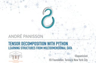
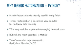


![from sklearn import datasets, decomposition, utils
digits = datasets.fetch_mldata('MNIST original')
A = utils.shuffle(digits.data)
nmf = decomposition.NMF(n_components=20)
W = nmf.fit_transform(A)
H = nmf.components_
plt.rc("image", cmap="binary")
plt.figure(figsize=(8,4))
for i in range(20):
plt.subplot(2,5,i+1)
plt.imshow(H[i].reshape(28,28))
plt.xticks(())
plt.yticks(())
plt.tight_layout()](https://image.slidesharecdn.com/pycon8-firenze-170409104152/85/TENSOR-DECOMPOSITION-WITH-PYTHON-11-320.jpg)
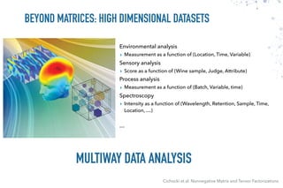


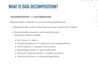
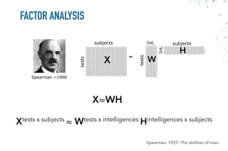
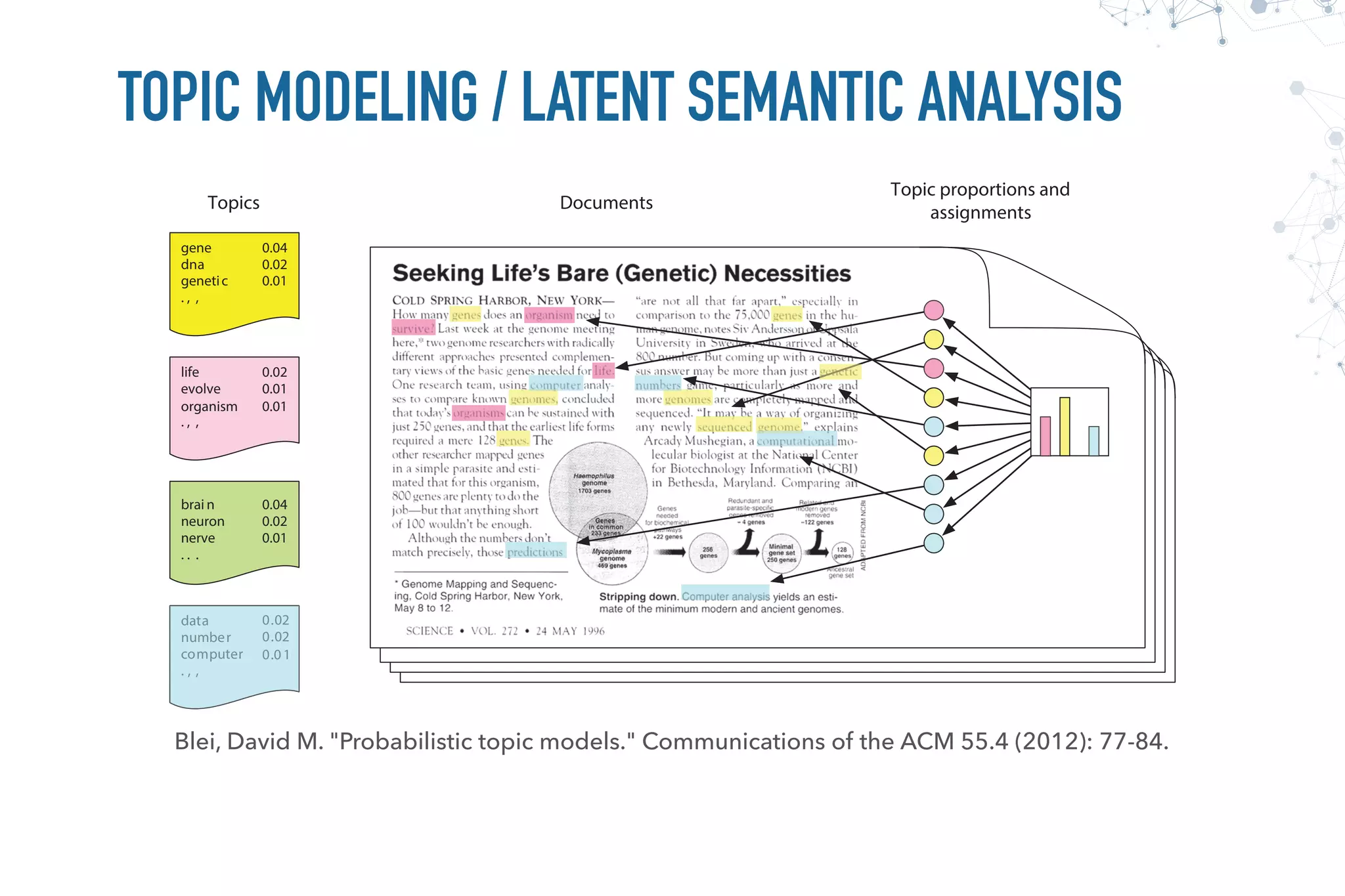
![FIBERS AND SLICES
Cichocki et al. Nonnegative Matrix and Tensor Factorizations
Column (Mode-1) Fibers Row (Mode-2) Fibers Tube (Mode-3) Fibers
Horizontal Slices Lateral Slices Frontal Slices
A[:, 4, 1] A[1, :, 4] A[1, 3, :]
A[1, :, :] A[:, :, 1]A[:, 1, :]](https://image.slidesharecdn.com/pycon8-firenze-170409104152/85/TENSOR-DECOMPOSITION-WITH-PYTHON-18-320.jpg)

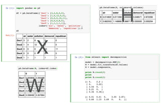
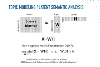
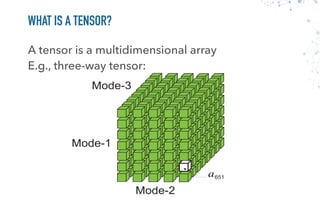
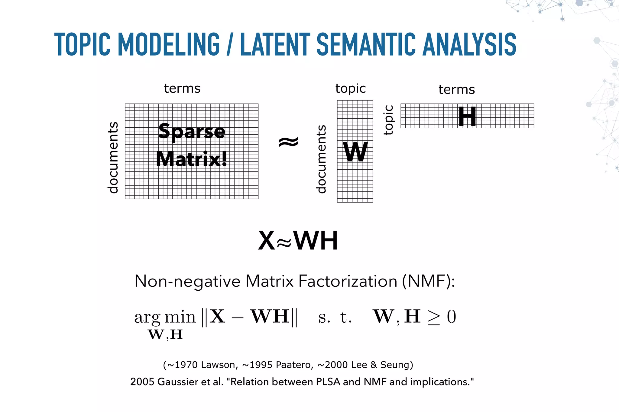
![>>> T = np.arange(0, 24).reshape((3, 4, 2))
>>> T
array([[[ 0, 1],
[ 2, 3],
[ 4, 5],
[ 6, 7]],
[[ 8, 9],
[10, 11],
[12, 13],
[14, 15]],
[[16, 17],
[18, 19],
[20, 21],
[22, 23]]])
OK for dense tensors: use a combination
of transpose() and reshape()
Not simple for sparse datasets (e.g.: <authors, terms, time>)
for j in range(T.shape[1]):
for i in range(T.shape[2]):
print T[:, i, j]
[ 0 8 16]
[ 2 10 18]
[ 4 12 20]
[ 6 14 22]
[ 1 9 17]
[ 3 11 19]
[ 5 13 21]
[ 7 15 23]
# supposing the existence of unfold
>>> T.unfold(0)
array([[ 0, 2, 4, 6, 1, 3, 5, 7],
[ 8, 10, 12, 14, 9, 11, 13, 15],
[16, 18, 20, 22, 17, 19, 21, 23]])
>>> T.unfold(1)
array([[ 0, 8, 16, 1, 9, 17],
[ 2, 10, 18, 3, 11, 19],
[ 4, 12, 20, 5, 13, 21],
[ 6, 14, 22, 7, 15, 23]])
>>> T.unfold(2)
array([[ 0, 8, 16, 2, 10, 18, 4, 12, 20, 6, 14, 22],
[ 1, 9, 17, 3, 11, 19, 5, 13, 21, 7, 15, 23]])](https://image.slidesharecdn.com/pycon8-firenze-170409104152/85/TENSOR-DECOMPOSITION-WITH-PYTHON-20-320.jpg)
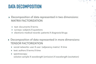
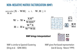
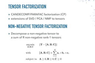
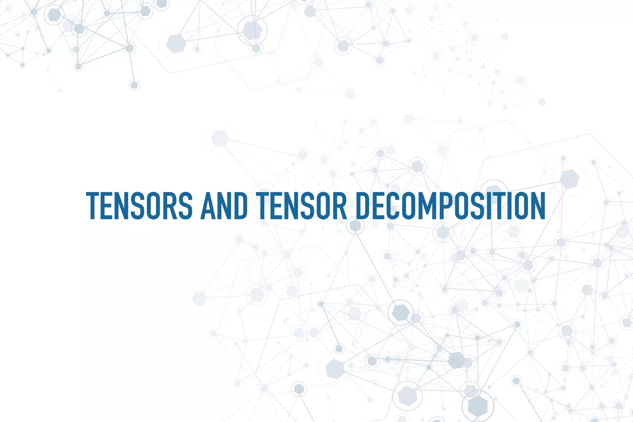
![RANK-1 TENSOR
The outer product of N vectors results in a rank-1 tensor
array([[[ 1., 2.],
[ 2., 4.],
[ 3., 6.],
[ 4., 8.]],
[[ 2., 4.],
[ 4., 8.],
[ 6., 12.],
[ 8., 16.]],
[[ 3., 6.],
[ 6., 12.],
[ 9., 18.],
[ 12., 24.]]])
a = np.array([1, 2, 3])
b = np.array([1, 2, 3, 4])
c = np.array([1, 2])
T = np.zeros((a.shape[0], b.shape[0], c.shape[0]))
for i in range(a.shape[0]):
for j in range(b.shape[0]):
for k in range(c.shape[0]):
T[i, j, k] = a[i] * b[j] * c[k]
T = a(1)
· · · a(N)
=
a
c
b
Ti,j,k = a
(1)
i a
(2)
j a
(3)
k](https://image.slidesharecdn.com/pycon8-firenze-170409104152/85/TENSOR-DECOMPOSITION-WITH-PYTHON-21-320.jpg)

![array([[[ 61., 82.],
[ 74., 100.],
[ 87., 118.],
[ 100., 136.]],
[[ 77., 104.],
[ 94., 128.],
[ 111., 152.],
[ 128., 176.]],
[[ 93., 126.],
[ 114., 156.],
[ 135., 186.],
[ 156., 216.]]])
A = np.array([[1, 2, 3],
[4, 5, 6]]).T
B = np.array([[1, 2, 3, 4],
[5, 6, 7, 8]]).T
C = np.array([[1, 2],
[3, 4]]).T
T = np.zeros((A.shape[0], B.shape[0], C.shape[0]))
for i in range(A.shape[0]):
for j in range(B.shape[0]):
for k in range(C.shape[0]):
for r in range(A.shape[1]):
T[i, j, k] += A[i, r] * B[j, r] * C[k, r]
T = np.einsum('ir,jr,kr->ijk', A, B, C)
: Kruskal Tensorbr cr ⌘ JA, B, CK](https://image.slidesharecdn.com/pycon8-firenze-170409104152/85/TENSOR-DECOMPOSITION-WITH-PYTHON-23-320.jpg)
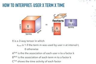
![TENSOR FACTORIZATION: HOW TO
Alternating Least Squares(ALS):
Fix all but one factor matrix to which LS is applied
min
A 0
kT(1) A(C B)T
k
min
B 0
kT(2) B(C A)T
k
min
C 0
kT(3) C(B A)T
k
denotes the Khatri-Rao product, which is a
column-wise Kronecker product, i.e., C B = [c1 ⌦ b1, c2 ⌦ b2, . . . , cr ⌦ br]
T(1) = ˆA(ˆC ˆB)T
T(2) = ˆB(ˆC ˆA)T
T(3) = ˆC(ˆB ˆA)T
Unfolded Tensor
on the kth mode](https://image.slidesharecdn.com/pycon8-firenze-170409104152/85/TENSOR-DECOMPOSITION-WITH-PYTHON-25-320.jpg)
![F = [zeros(n, r), zeros(m, r), zeros(o, r)]
FF_init = np.rand((len(F), r, r))
def iter_solver(T, F, FF_init):
# Update each factor
for k in range(len(F)):
# Compute the inner-product matrix
FF = ones((r, r))
for i in range(k) + range(k+1, len(F)):
FF = FF * FF_init[i]
# unfolded tensor times Khatri-Rao product
XF = T.uttkrp(F, k)
F[k] = F[k]*XF/(F[k].dot(FF))
# F[k] = nnls(FF, XF.T).T
FF_init[k] = (F[k].T.dot(F[k]))
return F, FF_init
min
A 0
kT(1) A(C B)T
k
min
B 0
kT(2) B(C A)T
k
min
C 0
kT(3) C(B A)T
k
arg min
W,H
kX WHk s.
J. Kim and H. Park. Fast Nonnegative Tensor Factorization with an Active-set-like Method.
In High-Performance Scientific Computing: Algorithms and Applications, Springer, 2012, pp. 311-326.
W W •
XHT
WHHT
T(1)(C B)](https://image.slidesharecdn.com/pycon8-firenze-170409104152/85/TENSOR-DECOMPOSITION-WITH-PYTHON-26-320.jpg)


![from sklearn import datasets, decomposition, utils
digits = datasets.fetch_mldata('MNIST original')
A = utils.shuffle(digits.data)
nmf = decomposition.NMF(n_components=20)
W = nmf.fit_transform(A)
H = nmf.components_
plt.rc("image", cmap="binary")
plt.figure(figsize=(8,4))
for i in range(20):
plt.subplot(2,5,i+1)
plt.imshow(H[i].reshape(28,28))
plt.xticks(())
plt.yticks(())
plt.tight_layout()](https://image.slidesharecdn.com/pycon8-firenze-170409104152/75/TENSOR-DECOMPOSITION-WITH-PYTHON-11-2048.jpg)


![FIBERS AND SLICES
Cichocki et al. Nonnegative Matrix and Tensor Factorizations
Column (Mode-1) Fibers Row (Mode-2) Fibers Tube (Mode-3) Fibers
Horizontal Slices Lateral Slices Frontal Slices
A[:, 4, 1] A[1, :, 4] A[1, 3, :]
A[1, :, :] A[:, :, 1]A[:, 1, :]](https://image.slidesharecdn.com/pycon8-firenze-170409104152/75/TENSOR-DECOMPOSITION-WITH-PYTHON-18-2048.jpg)
![>>> T = np.arange(0, 24).reshape((3, 4, 2))
>>> T
array([[[ 0, 1],
[ 2, 3],
[ 4, 5],
[ 6, 7]],
[[ 8, 9],
[10, 11],
[12, 13],
[14, 15]],
[[16, 17],
[18, 19],
[20, 21],
[22, 23]]])
OK for dense tensors: use a combination
of transpose() and reshape()
Not simple for sparse datasets (e.g.: <authors, terms, time>)
for j in range(T.shape[1]):
for i in range(T.shape[2]):
print T[:, i, j]
[ 0 8 16]
[ 2 10 18]
[ 4 12 20]
[ 6 14 22]
[ 1 9 17]
[ 3 11 19]
[ 5 13 21]
[ 7 15 23]
# supposing the existence of unfold
>>> T.unfold(0)
array([[ 0, 2, 4, 6, 1, 3, 5, 7],
[ 8, 10, 12, 14, 9, 11, 13, 15],
[16, 18, 20, 22, 17, 19, 21, 23]])
>>> T.unfold(1)
array([[ 0, 8, 16, 1, 9, 17],
[ 2, 10, 18, 3, 11, 19],
[ 4, 12, 20, 5, 13, 21],
[ 6, 14, 22, 7, 15, 23]])
>>> T.unfold(2)
array([[ 0, 8, 16, 2, 10, 18, 4, 12, 20, 6, 14, 22],
[ 1, 9, 17, 3, 11, 19, 5, 13, 21, 7, 15, 23]])](https://image.slidesharecdn.com/pycon8-firenze-170409104152/75/TENSOR-DECOMPOSITION-WITH-PYTHON-20-2048.jpg)
![RANK-1 TENSOR
The outer product of N vectors results in a rank-1 tensor
array([[[ 1., 2.],
[ 2., 4.],
[ 3., 6.],
[ 4., 8.]],
[[ 2., 4.],
[ 4., 8.],
[ 6., 12.],
[ 8., 16.]],
[[ 3., 6.],
[ 6., 12.],
[ 9., 18.],
[ 12., 24.]]])
a = np.array([1, 2, 3])
b = np.array([1, 2, 3, 4])
c = np.array([1, 2])
T = np.zeros((a.shape[0], b.shape[0], c.shape[0]))
for i in range(a.shape[0]):
for j in range(b.shape[0]):
for k in range(c.shape[0]):
T[i, j, k] = a[i] * b[j] * c[k]
T = a(1)
· · · a(N)
=
a
c
b
Ti,j,k = a
(1)
i a
(2)
j a
(3)
k](https://image.slidesharecdn.com/pycon8-firenze-170409104152/75/TENSOR-DECOMPOSITION-WITH-PYTHON-21-2048.jpg)
![array([[[ 61., 82.],
[ 74., 100.],
[ 87., 118.],
[ 100., 136.]],
[[ 77., 104.],
[ 94., 128.],
[ 111., 152.],
[ 128., 176.]],
[[ 93., 126.],
[ 114., 156.],
[ 135., 186.],
[ 156., 216.]]])
A = np.array([[1, 2, 3],
[4, 5, 6]]).T
B = np.array([[1, 2, 3, 4],
[5, 6, 7, 8]]).T
C = np.array([[1, 2],
[3, 4]]).T
T = np.zeros((A.shape[0], B.shape[0], C.shape[0]))
for i in range(A.shape[0]):
for j in range(B.shape[0]):
for k in range(C.shape[0]):
for r in range(A.shape[1]):
T[i, j, k] += A[i, r] * B[j, r] * C[k, r]
T = np.einsum('ir,jr,kr->ijk', A, B, C)
: Kruskal Tensorbr cr ⌘ JA, B, CK](https://image.slidesharecdn.com/pycon8-firenze-170409104152/75/TENSOR-DECOMPOSITION-WITH-PYTHON-23-2048.jpg)
![TENSOR FACTORIZATION: HOW TO
Alternating Least Squares(ALS):
Fix all but one factor matrix to which LS is applied
min
A 0
kT(1) A(C B)T
k
min
B 0
kT(2) B(C A)T
k
min
C 0
kT(3) C(B A)T
k
denotes the Khatri-Rao product, which is a
column-wise Kronecker product, i.e., C B = [c1 ⌦ b1, c2 ⌦ b2, . . . , cr ⌦ br]
T(1) = ˆA(ˆC ˆB)T
T(2) = ˆB(ˆC ˆA)T
T(3) = ˆC(ˆB ˆA)T
Unfolded Tensor
on the kth mode](https://image.slidesharecdn.com/pycon8-firenze-170409104152/75/TENSOR-DECOMPOSITION-WITH-PYTHON-25-2048.jpg)
![F = [zeros(n, r), zeros(m, r), zeros(o, r)]
FF_init = np.rand((len(F), r, r))
def iter_solver(T, F, FF_init):
# Update each factor
for k in range(len(F)):
# Compute the inner-product matrix
FF = ones((r, r))
for i in range(k) + range(k+1, len(F)):
FF = FF * FF_init[i]
# unfolded tensor times Khatri-Rao product
XF = T.uttkrp(F, k)
F[k] = F[k]*XF/(F[k].dot(FF))
# F[k] = nnls(FF, XF.T).T
FF_init[k] = (F[k].T.dot(F[k]))
return F, FF_init
min
A 0
kT(1) A(C B)T
k
min
B 0
kT(2) B(C A)T
k
min
C 0
kT(3) C(B A)T
k
arg min
W,H
kX WHk s.
J. Kim and H. Park. Fast Nonnegative Tensor Factorization with an Active-set-like Method.
In High-Performance Scientific Computing: Algorithms and Applications, Springer, 2012, pp. 311-326.
W W •
XHT
WHHT
T(1)(C B)](https://image.slidesharecdn.com/pycon8-firenze-170409104152/75/TENSOR-DECOMPOSITION-WITH-PYTHON-26-2048.jpg)
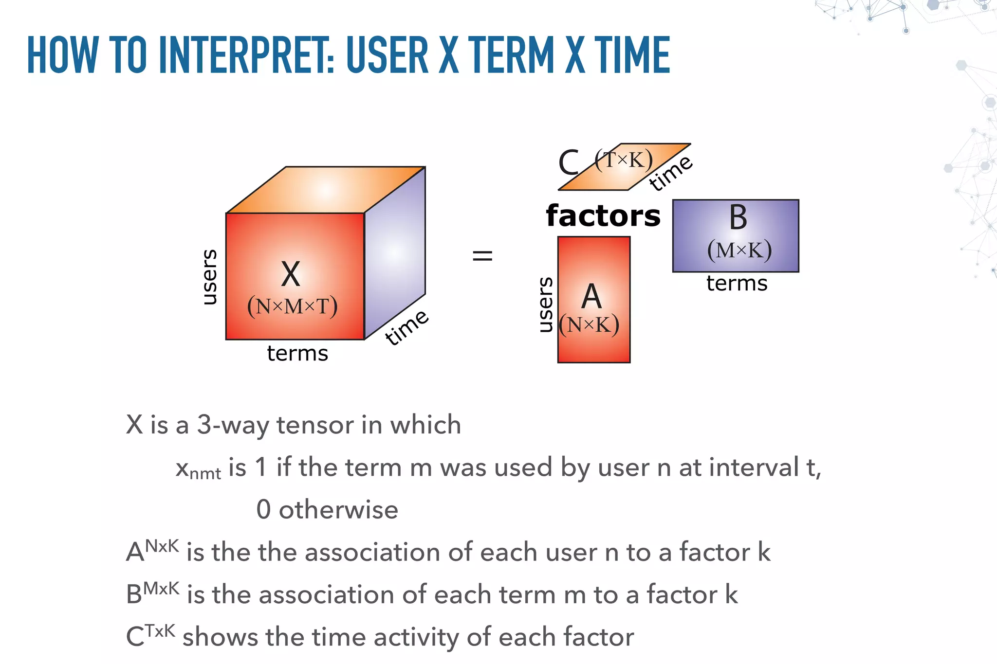


This document discusses tensor decomposition with Python. It begins by explaining what tensor decomposition and factorization are, and how they can be used to represent multi-dimensional datasets and perform dimensionality reduction. It then discusses matrix and tensor factorization methods like NMF, topic modeling, and CP/PARAFAC decomposition. The remainder of the document provides examples of tensor decomposition using Python tools and libraries, and discusses applications to analyzing temporal network and sensor data.
Introduction to tensor decomposition focusing on learning structures from multidimensional data.
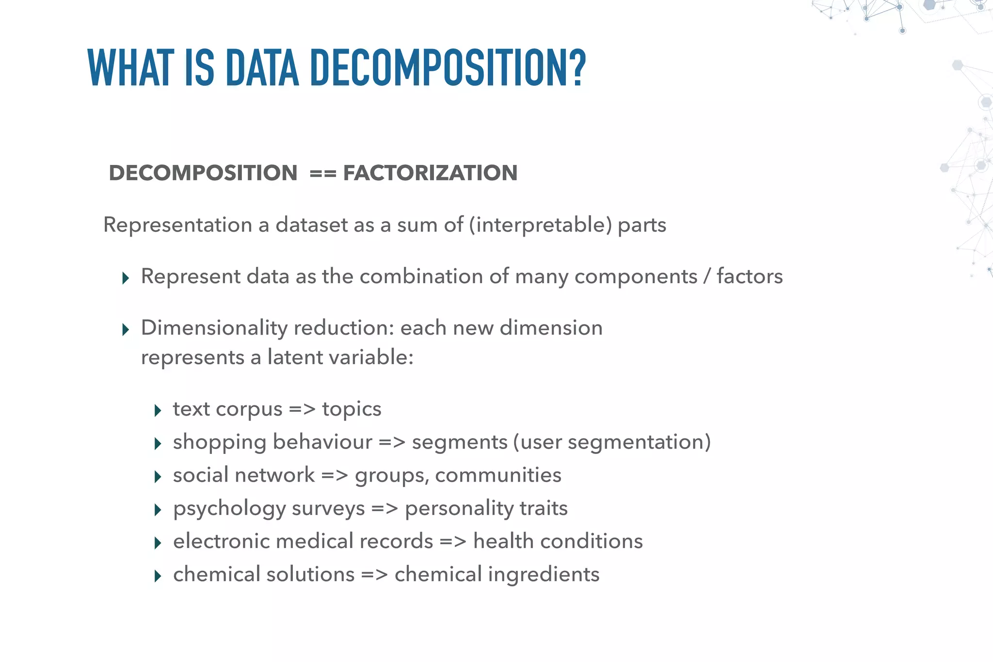
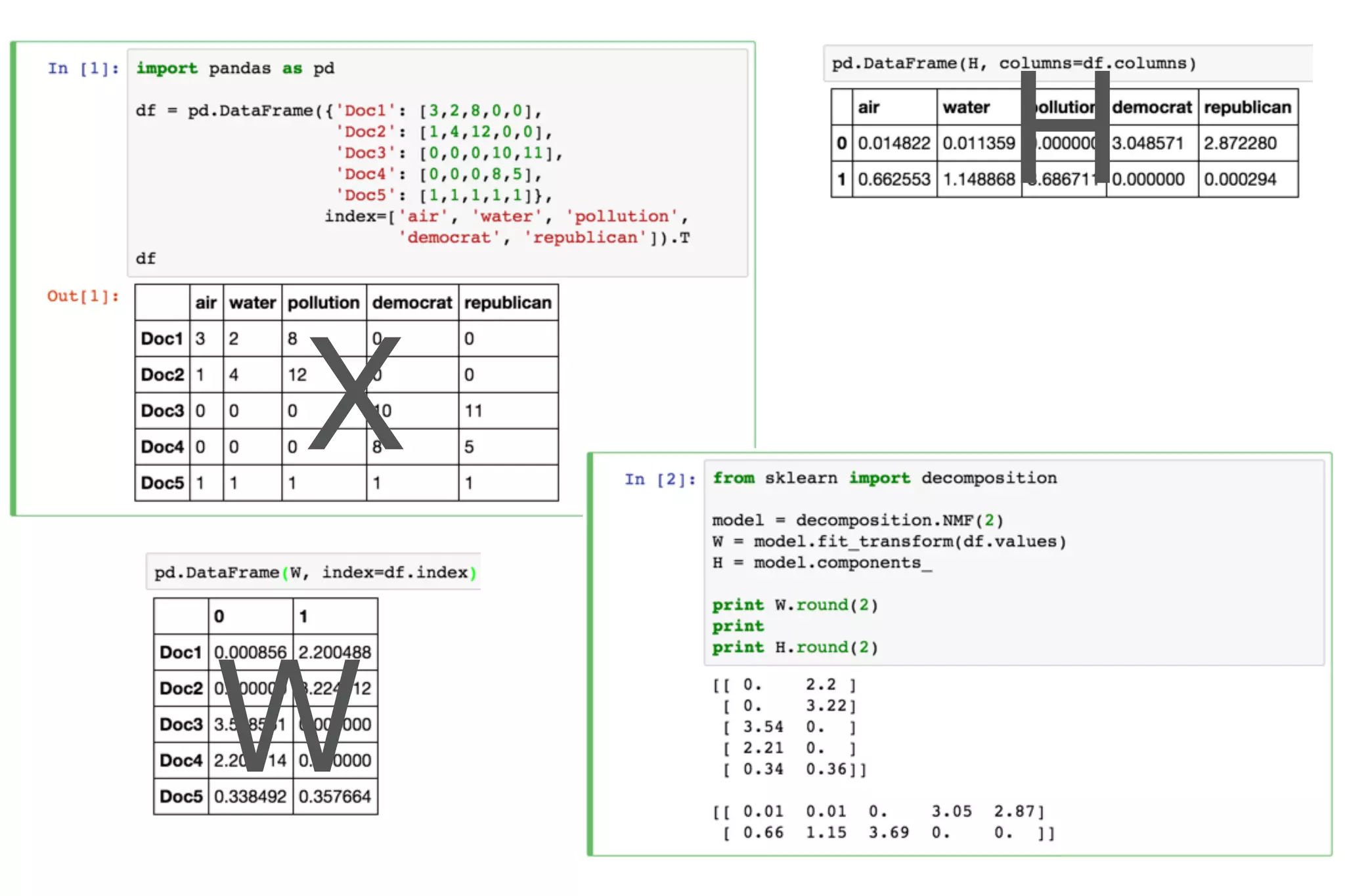
Explains data decomposition as factorization, covering matrix and tensor factorization with examples.
Discusses the significance of tensor factorization in multiway data analysis and its relation to matrix factorization.
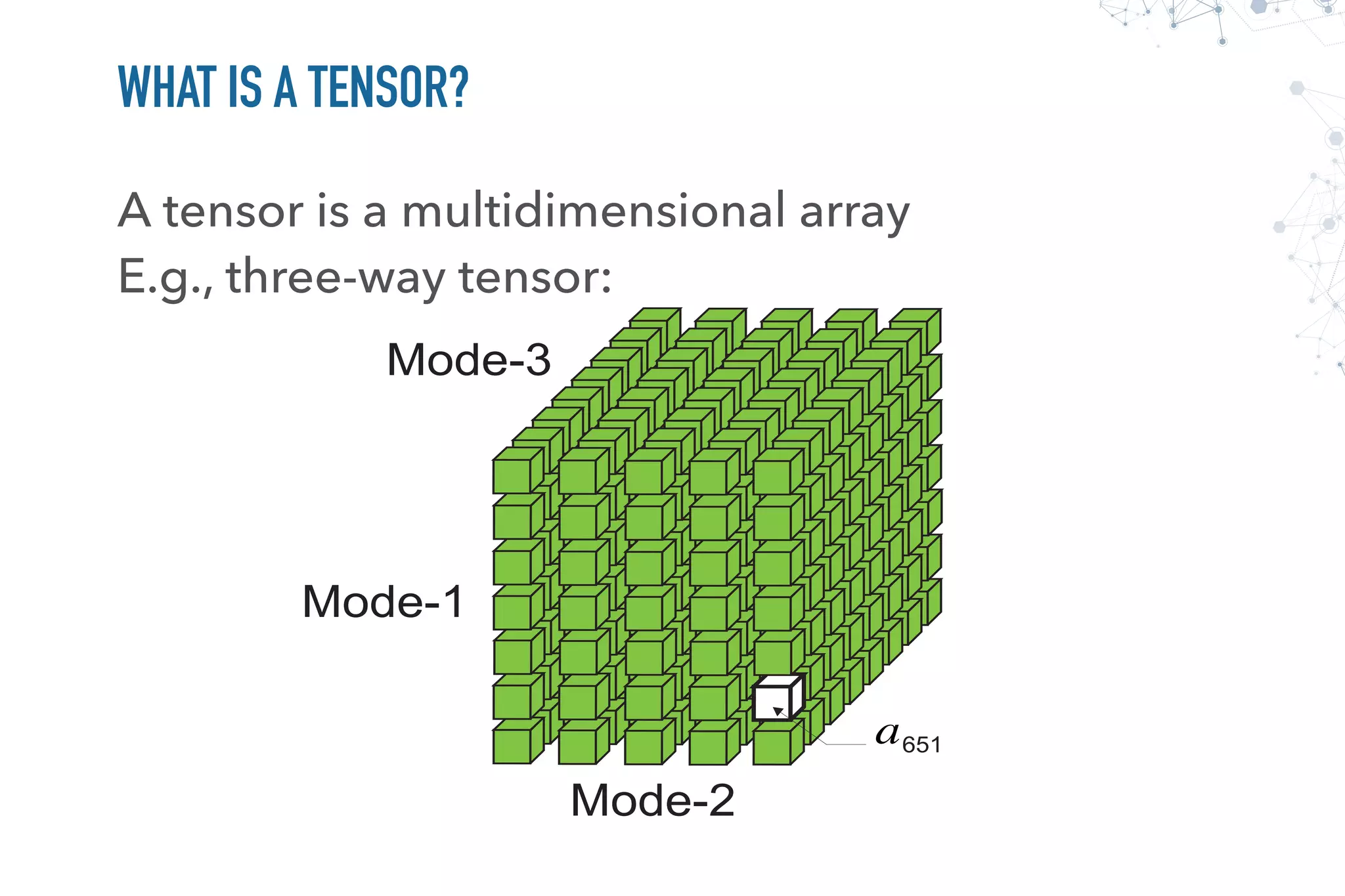
Introduction to tensors, their definition, and how tensor decomposition operates in high-dimensional datasets.
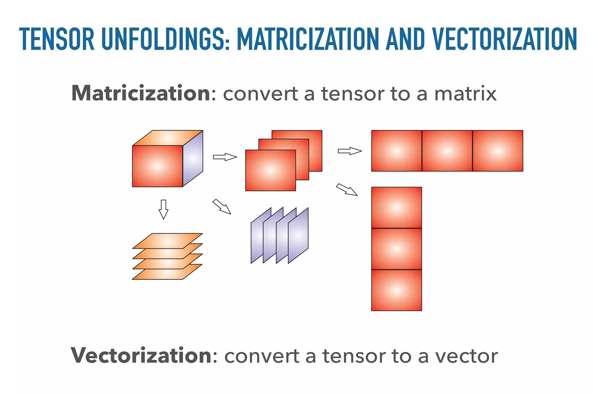
Examines the structure of tensors, including fibers, slices, and various tensor calculations such as unfolding.
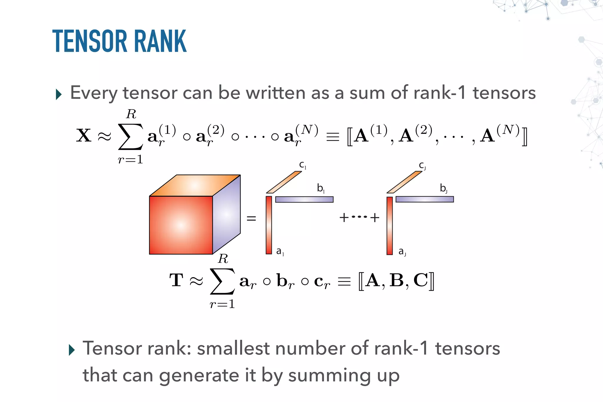
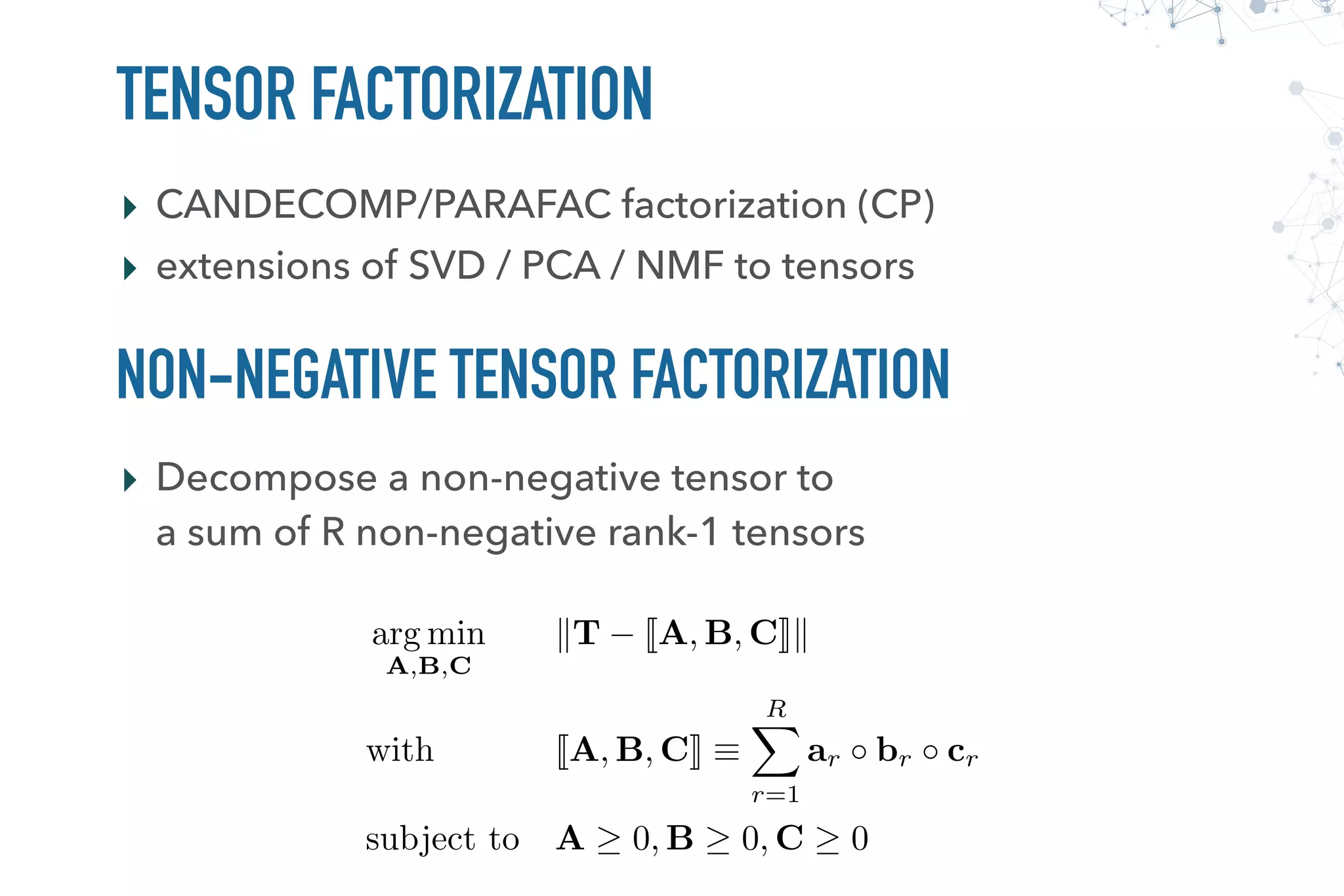
Discussion on tensor rank, tensor factorization techniques like CANDECOMP/PARAFAC and their implementation.
Approaches to interpret results from tensor analyses, including tools available in Python for tensor decomposition.
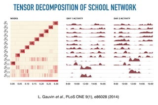
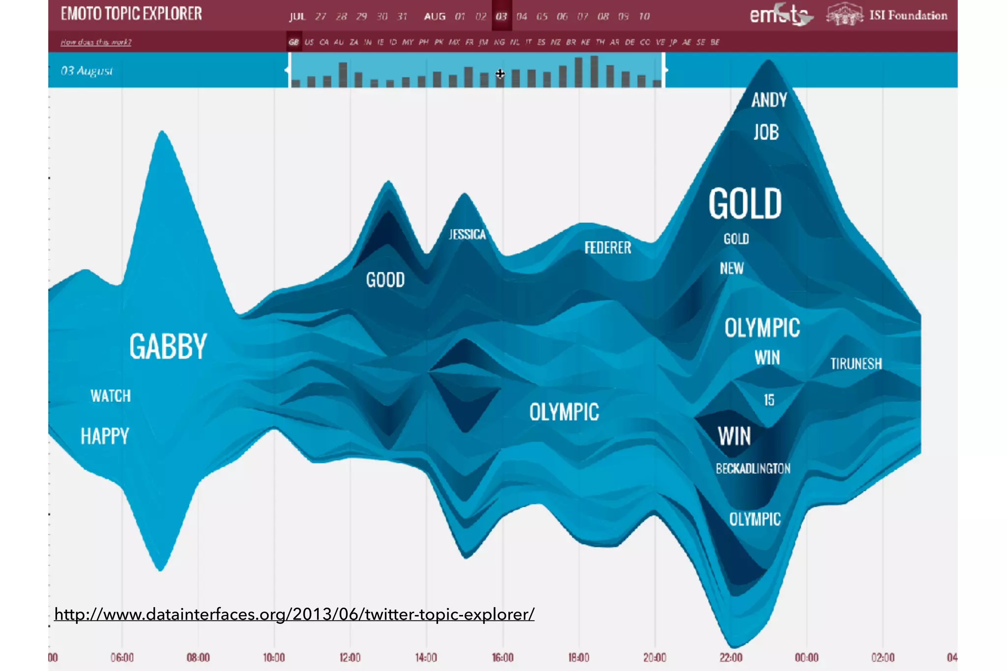
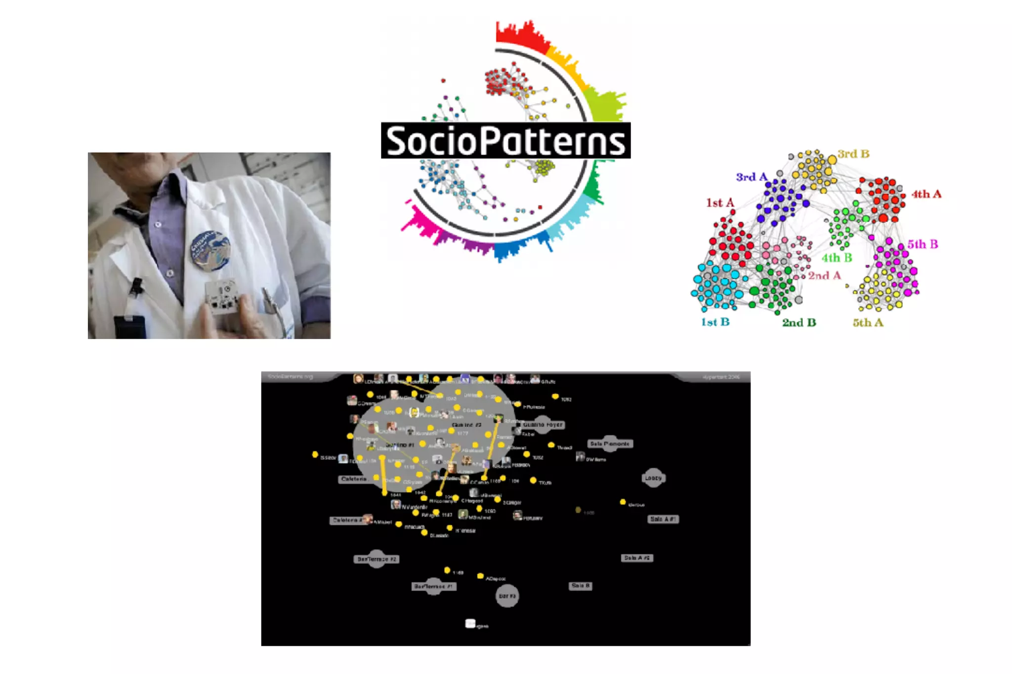
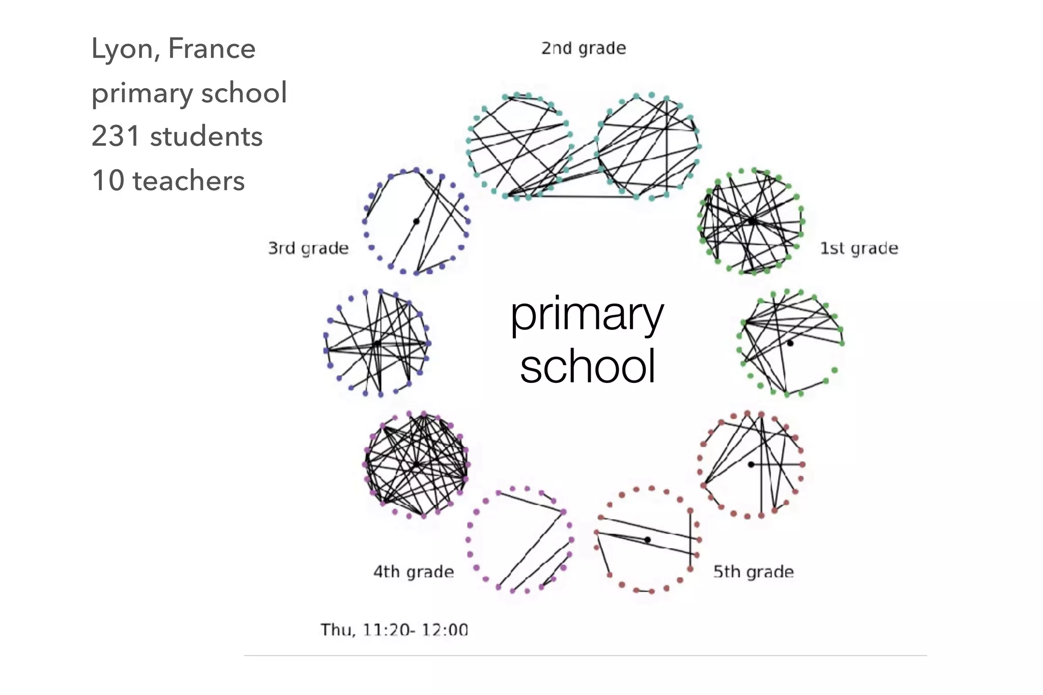
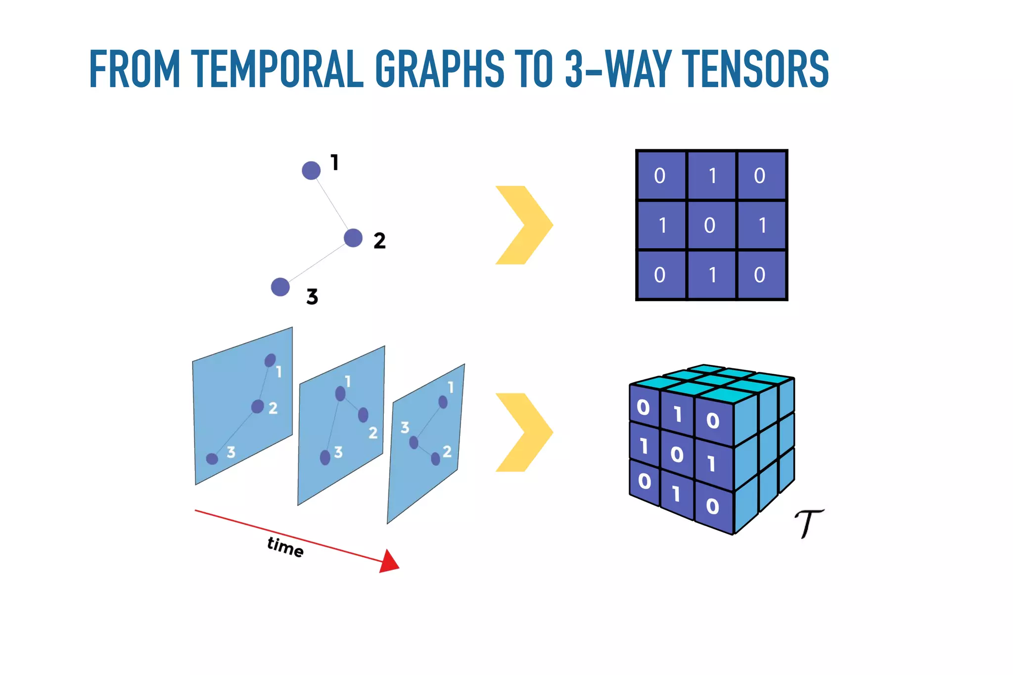
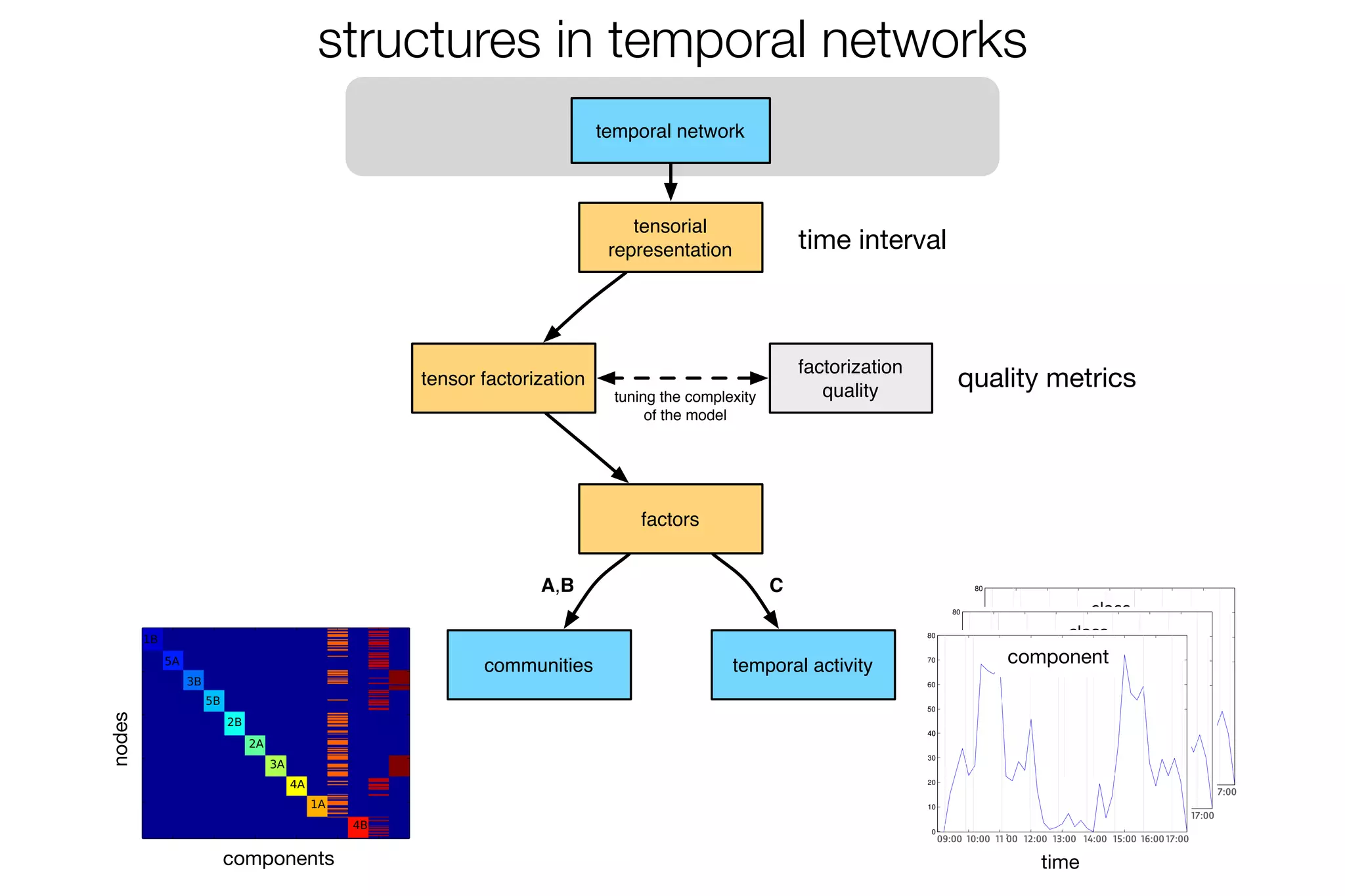
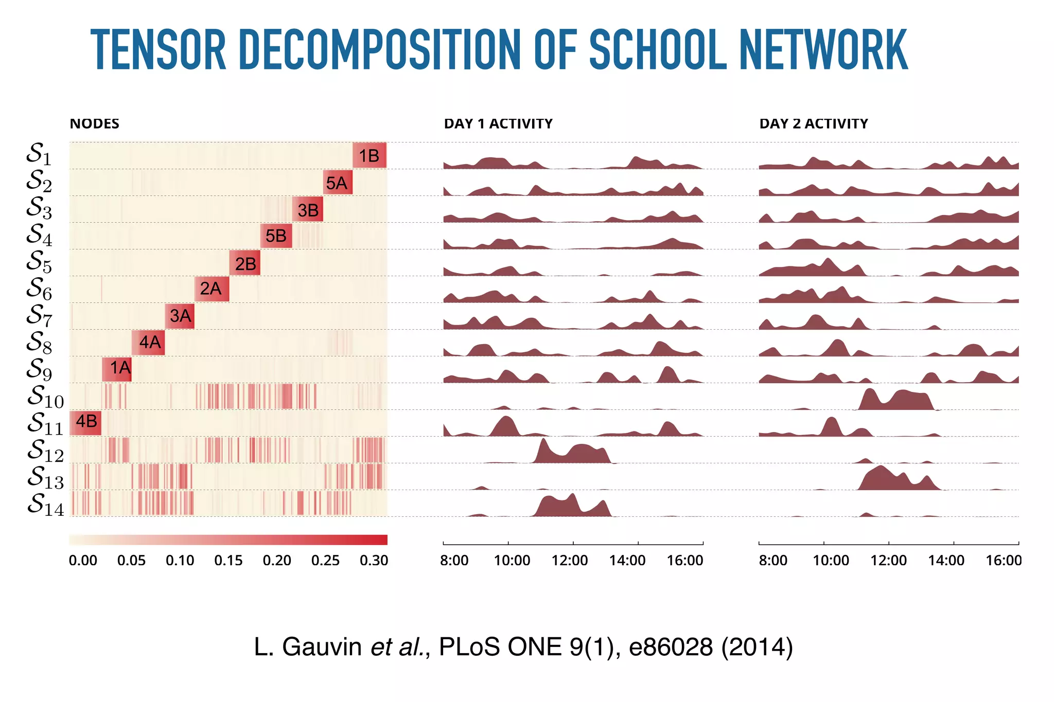
Applications of tensor decomposition in sensor data analysis, school network analysis, and examples for practical understanding.


