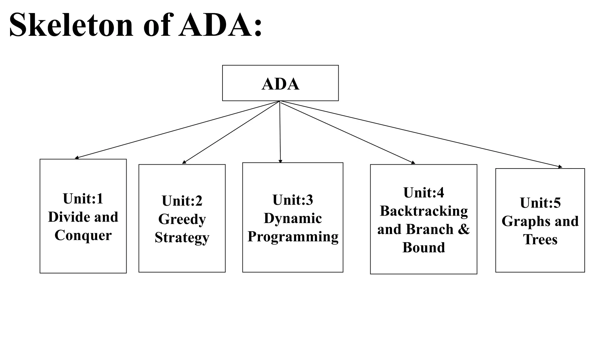
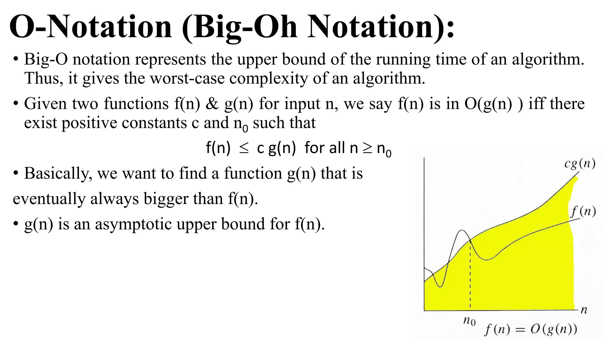
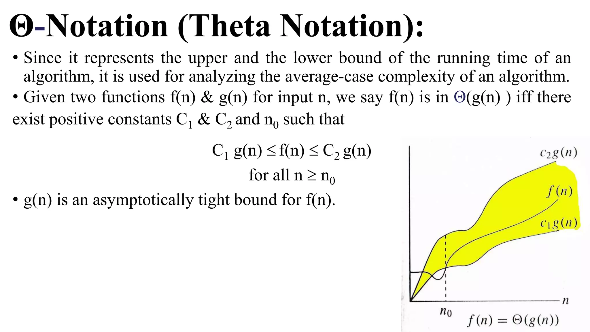
KEMBAR78
Analysis and Design of Algorithms | PPTX
Introduction to
Analysis & Design of Algorithm
Submitted by:
Prof. Bulbul Agrawal
Assistant Professor
Department of Computer Science & Engineering and Information Technology
Content
• Terminologies
• Course Objective
• Skeleton of the ADA
• Introduction to ADA
• Asymptotic Notations
• Algorithm Design Techniques
Terminologies:
• Algorithm Design:
Methods for designing efficient algorithms.
• Algorithm Analysis:
Analysis of resource usage of given algorithms. (Time & Space)
Why do we study this subject?
• Efficient algorithms lead to efficient programs.
• Efficient programs sell better.
• Efficient programs make better used of hardware.
• Programmers who write efficient programs are preferred.
Course Objective:
• The data structure includes analyzing various algorithms along with time and space
complexities. It also helps students to design new algorithms through mathematical
analysis and programming.
Skeleton of ADA:
ADA
Unit:1
Divide and
Conquer
Unit:2
Greedy
Strategy
Unit:3
Dynamic
Programming
Unit:4
Backtracking
and Branch &
Bound
Unit:5
Graphs and
Trees
Introduction:
• The set of rules that define how a particular problem can be solved in finite number of
steps is known as algorithm.
• An algorithm is a list of steps (Sequence of unambiguous instructions) for solving a
problem that transforms the input into the output.
Problem
Algorithm
Computer
Input Output
Designing of an algorithm:
Understand the problem
Decision making on:
Capabilities of computational devices
Algorithm Design Techniques
Data Structures
Specification of algorithms
Analysis of algorithm
Algorithm verification
Code the algorithm
Properties of an algorithm:
• An algorithm takes zero or more inputs.
• An algorithm results in one or more outputs.
• All operations can be carried out in a finite amount of time.
• An algorithm should be efficient and flexible.
• It should use less memory space as much as possible.
• An algorithm must terminate after a finite number of steps.
• Each step in the algorithm must be easily understood.
• An algorithm should be concise and compact to facilitate verification of their
correctness.
Two main tasks in the study of Algorithms:
• Algorithm Design
• Analysis of Algorithms
How to analyzed the algorithm?
Algorithm efficiency can be measured by two aspects;
Time Complexity: Given in terms of frequency count
• Instructions take time.
• How fast does the algorithm perform?
• What affects its runtime?
Space Complexity: Amount of memory required
• Data structure take space.
• What kind of data structure can be used?
• How does choice of data structure affect the runtime?
Asymptotic Notations:
 Given two algorithms for a task, how we find out which one is better?
1. It might be possible that for some inputs, first algorithm performs better than
the second. And for some inputs second performs better.
2. Or it might also be possible that for some inputs, first algorithm perform
better on one machine and the second works better on other machine for
some other inputs.
 So Asymptotic Notation is the big idea that handles above issues in analysing
algorithms. In Asymptotic Analysis, we evaluate the performance of an
algorithm in terms of input size.
 Using Asymptotic Analysis we can very well conclude the Best Case, Average
Case, and Worst Case scenario of an algorithm.
Asymptotic Notations:
• Asymptotic Notations are used to represent the complexity of an algorithm.
• Asymptotic Notations provides with a mechanism to calculate and represent
time and space complexity for any algorithm.
Order of Growth:
• Order of growth in algorithm means how the time for computation increase
when you increase the input size. It really matters when your input size is very
large.
Kind of Analysis:
Usually the time required by an algorithm falls under three types:
 Best Case: Minimum time required for algorithm execution
 Average Case: Average time required for algorithm execution
 Worst Case: Worst time required for algorithm execution
Following are the commonly used asymptotic notations to calculate the running
time complexity of an algorithm;
 O-Notation (Big-Oh Notation)
 Ω-Notation (Omega Notation)
 Θ-Notation (Theta Notation)
O-Notation (Big-Oh Notation):
• Big-O notation represents the upper bound of the running time of an algorithm.
Thus, it gives the worst-case complexity of an algorithm.
• Given two functions f(n) & g(n) for input n, we say f(n) is in O(g(n) ) iff there
exist positive constants c and n0 such that
f(n) ļ‚£ c g(n) for all n  n0
• Basically, we want to find a function g(n) that is
eventually always bigger than f(n).
• g(n) is an asymptotic upper bound for f(n).
Ī©-Notation (Omega Notation):
• Omega notation represents the lower bound of the running time of an
algorithm. Thus, it provides the best case complexity of an algorithm.
• Given two functions f(n) & g(n) for input n, we say f(n) is in Ī©(g(n) ) iff there
exist positive constants c and n0 such that
f(n)  c g(n) for all n  n0
• Basically, we want to find a function g(n) that is
eventually always smaller than f(n).
• g(n) is an asymptotic lower bound for f(n).
Θ-Notation (Theta Notation):
• Since it represents the upper and the lower bound of the running time of an
algorithm, it is used for analyzing the average-case complexity of an algorithm.
• Given two functions f(n) & g(n) for input n, we say f(n) is in Θ(g(n) ) iff there
exist positive constants C1 & C2 and n0 such that
C1 g(n) ļ‚£ f(n) ļ‚£ C2 g(n)
for all n  n0
• g(n) is an asymptotically tight bound for f(n).
Algorithm Design Strategies:
We can design an algorithm by choose the one of the following strategies:
1. Divide and Conquer
2. Greedy Algorithm
3. Dynamic programming
4. Backtracking
5. Branch and Bound
1. Divide & Conquer Strategy:
The algorithm which follows divide and conquer technique involves 3 steps:
1. Divide the original problem into a set of sub problems.
2. Conquer (or solve) every sub-problem individually, recursive.
3. Combine the solutions of these sub problems to get the solution of original
problem.
 Problems that follow divide and conquer strategy:
• Merge Sort
• Binary Search
• Strassen's Matrix Multiplication
2. Greedy Strategy:
• Greedy technique is used to solve an optimization problem. (Repeatedly do what is
best now)
• An Optimization problem is one in which, we are given a set of input values, which
are required to be either maximized or minimized (known as objective function) w.r.t.
some constraints or conditions.
• The greedy algorithm does not always guarantee the optimal solution but it generally
produces solutions that are very close in value to the optimal.
 Problems that follow greedy strategy:
• Fractional Knapsack Problem
• Minimum Spanning Tress
• Single Source Shortest Path Algorithm
• Job Sequencing With Deadline
3. Dynamic Programming:
• Dynamic programming is a technique that breaks the problems into sub-
problems, and saves the result for future purposes so that we do not need to
compute the result again.
• The subproblems are optimized to optimize the overall solution is known as
optimal substructure property.
Problems that follow dynamic strategy:
• 0/1 Knapsack
• Matrix Chain Multiplication
• Multistage Graph
4. Backtracking:
• Backtracking is an algorithmic technique for solving problems by trying to
build a solution incrementally, one piece at a time, removing those solutions
that fail to satisfy the constraints of the problem at any point
• Backtracking is not used for optimization. Backtracking basically means trying
all possible options. It is used when you have multiple solution and you want
all those solutions.
Problems that follow backtracking strategy:
• N-Queen’s Problems
• Graph Colouring
• Hamiltonian Cycle
5. Branch and Bound:
• It is similar to the backtracking since it also uses the state space tree. It is used
for solving the optimization problems and minimization problems.
• A branch and bound algorithm is an optimization technique to get an optimal
solution to the problem. It looks for the best solution for a given problem in the
entire space of the solution. The bounds in the function to be optimized are
merged with the value of the latest best solution.
Problem that follow branch and bound strategy:
• Travelling Salesman Problem
After completion the course, Students will
be able to:
• Determine the time and space complexity of simple algorithms.
• Use notations to give upper, lower, and tight bounds on time and space
complexity of algorithms.
• Practice the main algorithm design strategies of Brute Force, Divide and
Conquer, Greedy Methods, Dynamic Programming, Backtracking, and Branch
and Bound and implement examples of each.
• Implement the most common sorting and searching algorithms and perform
their complexity analysis.
• Solve problems using the fundamental graph algorithms.
• Evaluate, select and implement algorithms in programming context.
Reference Books:
• Coremen Thomas, Leiserson CE, Rivest RL; Introduction to Algorithms; PHI.
• Horowitz & Sahani; Analysis & Design of Algorithm
• Dasgupta; algorithms; TMH
• Ullmann; Analysis & Design of Algorithm
• Michael T Goodrich, Robarto Tamassia, Algorithm Design, Wiely India
Analysis and Design of Algorithms

Analysis and Design of Algorithms

  • 1.
    Introduction to Analysis &Design of Algorithm Submitted by: Prof. Bulbul Agrawal Assistant Professor Department of Computer Science & Engineering and Information Technology
  • 2.
    Content • Terminologies • CourseObjective • Skeleton of the ADA • Introduction to ADA • Asymptotic Notations • Algorithm Design Techniques
  • 3.
    Terminologies: • Algorithm Design: Methodsfor designing efficient algorithms. • Algorithm Analysis: Analysis of resource usage of given algorithms. (Time & Space)
  • 4.
    Why do westudy this subject? • Efficient algorithms lead to efficient programs. • Efficient programs sell better. • Efficient programs make better used of hardware. • Programmers who write efficient programs are preferred.
  • 5.
    Course Objective: • Thedata structure includes analyzing various algorithms along with time and space complexities. It also helps students to design new algorithms through mathematical analysis and programming.
  • 6.
    Skeleton of ADA: ADA Unit:1 Divideand Conquer Unit:2 Greedy Strategy Unit:3 Dynamic Programming Unit:4 Backtracking and Branch & Bound Unit:5 Graphs and Trees
  • 7.
    Introduction: • The setof rules that define how a particular problem can be solved in finite number of steps is known as algorithm. • An algorithm is a list of steps (Sequence of unambiguous instructions) for solving a problem that transforms the input into the output. Problem Algorithm Computer Input Output
  • 8.
    Designing of analgorithm: Understand the problem Decision making on: Capabilities of computational devices Algorithm Design Techniques Data Structures Specification of algorithms Analysis of algorithm Algorithm verification Code the algorithm
  • 9.
    Properties of analgorithm: • An algorithm takes zero or more inputs. • An algorithm results in one or more outputs. • All operations can be carried out in a finite amount of time. • An algorithm should be efficient and flexible. • It should use less memory space as much as possible. • An algorithm must terminate after a finite number of steps. • Each step in the algorithm must be easily understood. • An algorithm should be concise and compact to facilitate verification of their correctness.
  • 10.
    Two main tasksin the study of Algorithms: • Algorithm Design • Analysis of Algorithms
  • 11.
    How to analyzedthe algorithm? Algorithm efficiency can be measured by two aspects; Time Complexity: Given in terms of frequency count • Instructions take time. • How fast does the algorithm perform? • What affects its runtime? Space Complexity: Amount of memory required • Data structure take space. • What kind of data structure can be used? • How does choice of data structure affect the runtime?
  • 12.
    Asymptotic Notations:  Giventwo algorithms for a task, how we find out which one is better? 1. It might be possible that for some inputs, first algorithm performs better than the second. And for some inputs second performs better. 2. Or it might also be possible that for some inputs, first algorithm perform better on one machine and the second works better on other machine for some other inputs.  So Asymptotic Notation is the big idea that handles above issues in analysing algorithms. In Asymptotic Analysis, we evaluate the performance of an algorithm in terms of input size.  Using Asymptotic Analysis we can very well conclude the Best Case, Average Case, and Worst Case scenario of an algorithm.
  • 13.
    Asymptotic Notations: • AsymptoticNotations are used to represent the complexity of an algorithm. • Asymptotic Notations provides with a mechanism to calculate and represent time and space complexity for any algorithm. Order of Growth: • Order of growth in algorithm means how the time for computation increase when you increase the input size. It really matters when your input size is very large.
  • 14.
    Kind of Analysis: Usuallythe time required by an algorithm falls under three types:  Best Case: Minimum time required for algorithm execution  Average Case: Average time required for algorithm execution  Worst Case: Worst time required for algorithm execution Following are the commonly used asymptotic notations to calculate the running time complexity of an algorithm;  O-Notation (Big-Oh Notation)  Ω-Notation (Omega Notation)  Θ-Notation (Theta Notation)
  • 15.
    O-Notation (Big-Oh Notation): •Big-O notation represents the upper bound of the running time of an algorithm. Thus, it gives the worst-case complexity of an algorithm. • Given two functions f(n) & g(n) for input n, we say f(n) is in O(g(n) ) iff there exist positive constants c and n0 such that f(n) ļ‚£ c g(n) for all n  n0 • Basically, we want to find a function g(n) that is eventually always bigger than f(n). • g(n) is an asymptotic upper bound for f(n).
  • 16.
    Ī©-Notation (Omega Notation): •Omega notation represents the lower bound of the running time of an algorithm. Thus, it provides the best case complexity of an algorithm. • Given two functions f(n) & g(n) for input n, we say f(n) is in Ī©(g(n) ) iff there exist positive constants c and n0 such that f(n)  c g(n) for all n  n0 • Basically, we want to find a function g(n) that is eventually always smaller than f(n). • g(n) is an asymptotic lower bound for f(n).
  • 17.
    Θ-Notation (Theta Notation): •Since it represents the upper and the lower bound of the running time of an algorithm, it is used for analyzing the average-case complexity of an algorithm. • Given two functions f(n) & g(n) for input n, we say f(n) is in Θ(g(n) ) iff there exist positive constants C1 & C2 and n0 such that C1 g(n) ļ‚£ f(n) ļ‚£ C2 g(n) for all n  n0 • g(n) is an asymptotically tight bound for f(n).
  • 18.
    Algorithm Design Strategies: Wecan design an algorithm by choose the one of the following strategies: 1. Divide and Conquer 2. Greedy Algorithm 3. Dynamic programming 4. Backtracking 5. Branch and Bound
  • 19.
    1. Divide &Conquer Strategy: The algorithm which follows divide and conquer technique involves 3 steps: 1. Divide the original problem into a set of sub problems. 2. Conquer (or solve) every sub-problem individually, recursive. 3. Combine the solutions of these sub problems to get the solution of original problem.  Problems that follow divide and conquer strategy: • Merge Sort • Binary Search • Strassen's Matrix Multiplication
  • 20.
    2. Greedy Strategy: •Greedy technique is used to solve an optimization problem. (Repeatedly do what is best now) • An Optimization problem is one in which, we are given a set of input values, which are required to be either maximized or minimized (known as objective function) w.r.t. some constraints or conditions. • The greedy algorithm does not always guarantee the optimal solution but it generally produces solutions that are very close in value to the optimal.  Problems that follow greedy strategy: • Fractional Knapsack Problem • Minimum Spanning Tress • Single Source Shortest Path Algorithm • Job Sequencing With Deadline
  • 21.
    3. Dynamic Programming: •Dynamic programming is a technique that breaks the problems into sub- problems, and saves the result for future purposes so that we do not need to compute the result again. • The subproblems are optimized to optimize the overall solution is known as optimal substructure property. Problems that follow dynamic strategy: • 0/1 Knapsack • Matrix Chain Multiplication • Multistage Graph
  • 22.
    4. Backtracking: • Backtrackingis an algorithmic technique for solving problems by trying to build a solution incrementally, one piece at a time, removing those solutions that fail to satisfy the constraints of the problem at any point • Backtracking is not used for optimization. Backtracking basically means trying all possible options. It is used when you have multiple solution and you want all those solutions. Problems that follow backtracking strategy: • N-Queen’s Problems • Graph Colouring • Hamiltonian Cycle
  • 23.
    5. Branch andBound: • It is similar to the backtracking since it also uses the state space tree. It is used for solving the optimization problems and minimization problems. • A branch and bound algorithm is an optimization technique to get an optimal solution to the problem. It looks for the best solution for a given problem in the entire space of the solution. The bounds in the function to be optimized are merged with the value of the latest best solution. Problem that follow branch and bound strategy: • Travelling Salesman Problem
  • 24.
    After completion thecourse, Students will be able to: • Determine the time and space complexity of simple algorithms. • Use notations to give upper, lower, and tight bounds on time and space complexity of algorithms. • Practice the main algorithm design strategies of Brute Force, Divide and Conquer, Greedy Methods, Dynamic Programming, Backtracking, and Branch and Bound and implement examples of each. • Implement the most common sorting and searching algorithms and perform their complexity analysis. • Solve problems using the fundamental graph algorithms. • Evaluate, select and implement algorithms in programming context.
  • 25.
    Reference Books: • CoremenThomas, Leiserson CE, Rivest RL; Introduction to Algorithms; PHI. • Horowitz & Sahani; Analysis & Design of Algorithm • Dasgupta; algorithms; TMH • Ullmann; Analysis & Design of Algorithm • Michael T Goodrich, Robarto Tamassia, Algorithm Design, Wiely India