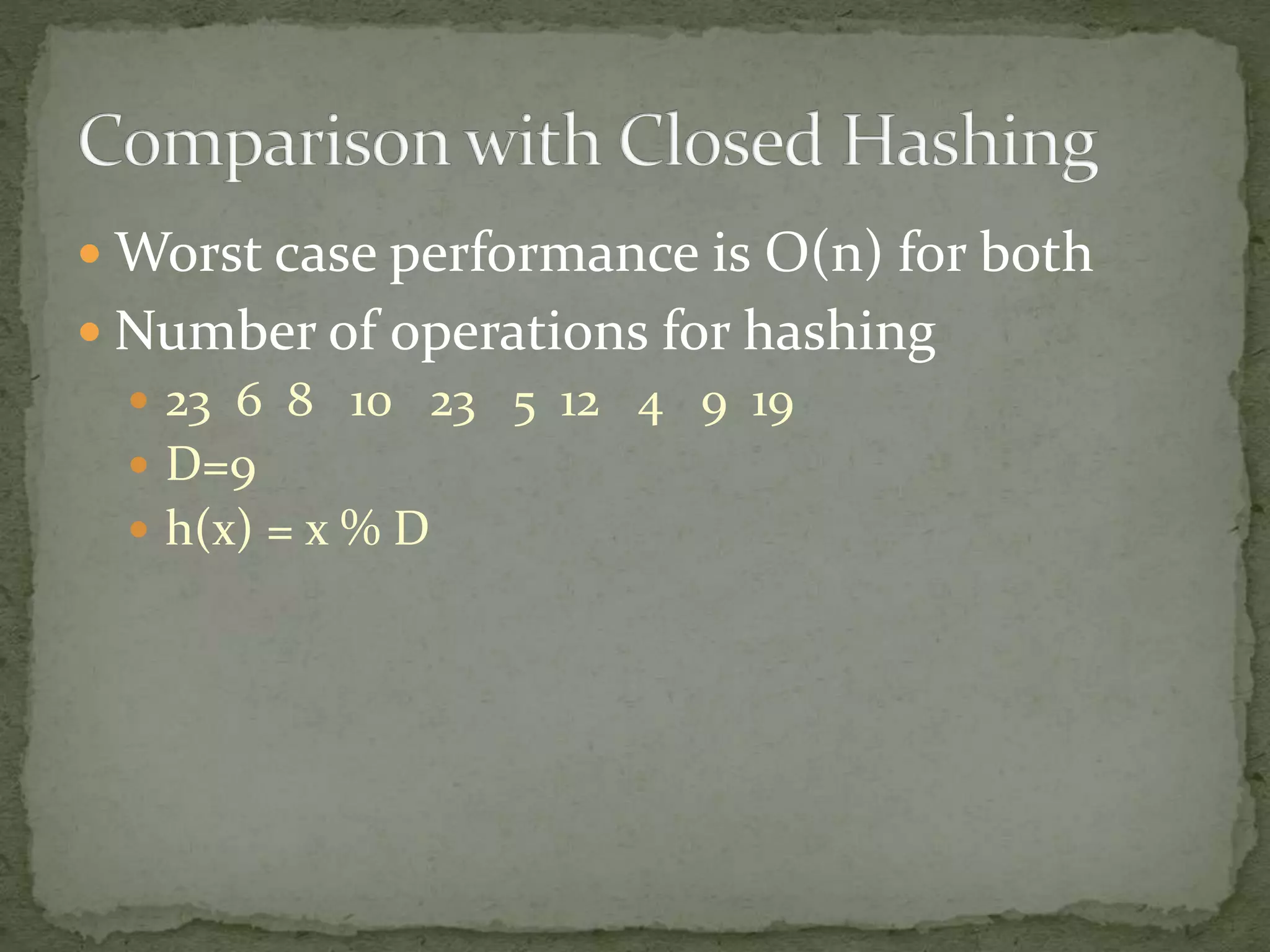
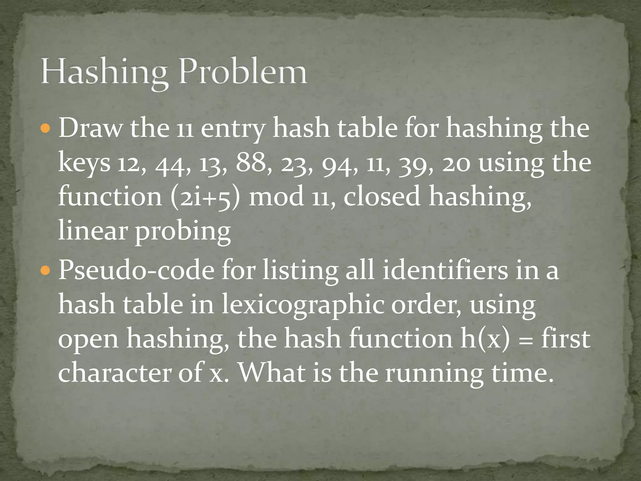
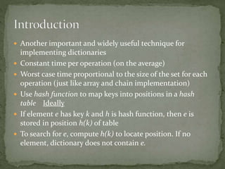
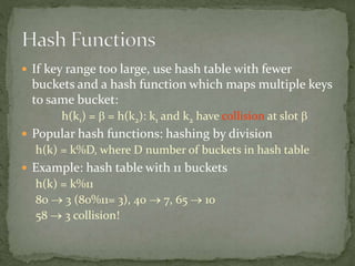
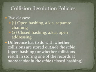
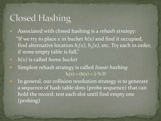
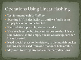
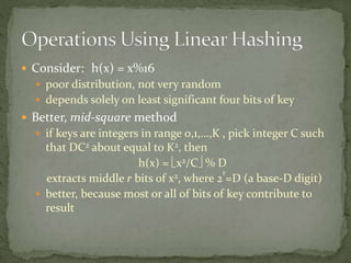
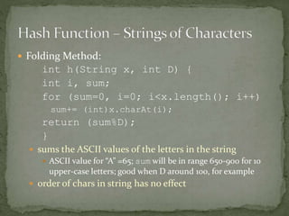
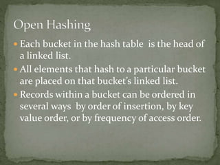
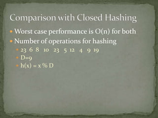
The document discusses hash tables and hashing techniques. It describes how hash tables use a hash function to map keys to positions in a table. Collisions can occur if multiple keys map to the same position. There are two main approaches to handling collisions - open hashing which stores collided items in linked lists, and closed hashing which uses techniques like linear probing to find alternate positions in the table. The document also discusses various hash functions and their properties, like minimizing collisions.
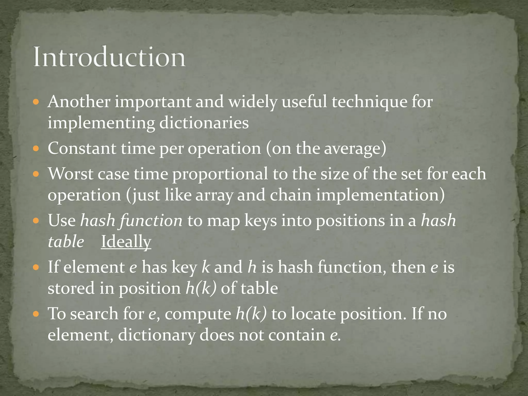
![Dictionary Student Records
Keys are ID numbers (951000 - 952000), no more
than 100 students
Hash function: h(k) = k-951000 maps ID into
distinct table positions 0-1000
array table[1001]
...
0 1 2 3 1000
hash table
buckets](https://image.slidesharecdn.com/hashingindatastructure-191003110849/85/Hashing-in-datastructure-3-320.jpg)


![Dictionary Student Records
Keys are ID numbers (951000 - 952000), no more
than 100 students
Hash function: h(k) = k-951000 maps ID into
distinct table positions 0-1000
array table[1001]
...
0 1 2 3 1000
hash table
buckets](https://image.slidesharecdn.com/hashingindatastructure-191003110849/75/Hashing-in-datastructure-3-2048.jpg)