Presentation on Greedy Algorithm process.ppt

ICT-307
Design & Analysis of Algorithms
Greedy Algorithms

2
Greedy Algorithm
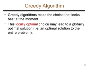
• Greedy algorithms make the choice that looks
best at the moment.
• This locally optimal choice may lead to a globally
optimal solution (i.e. an optimal solution to the
entire problem).

3
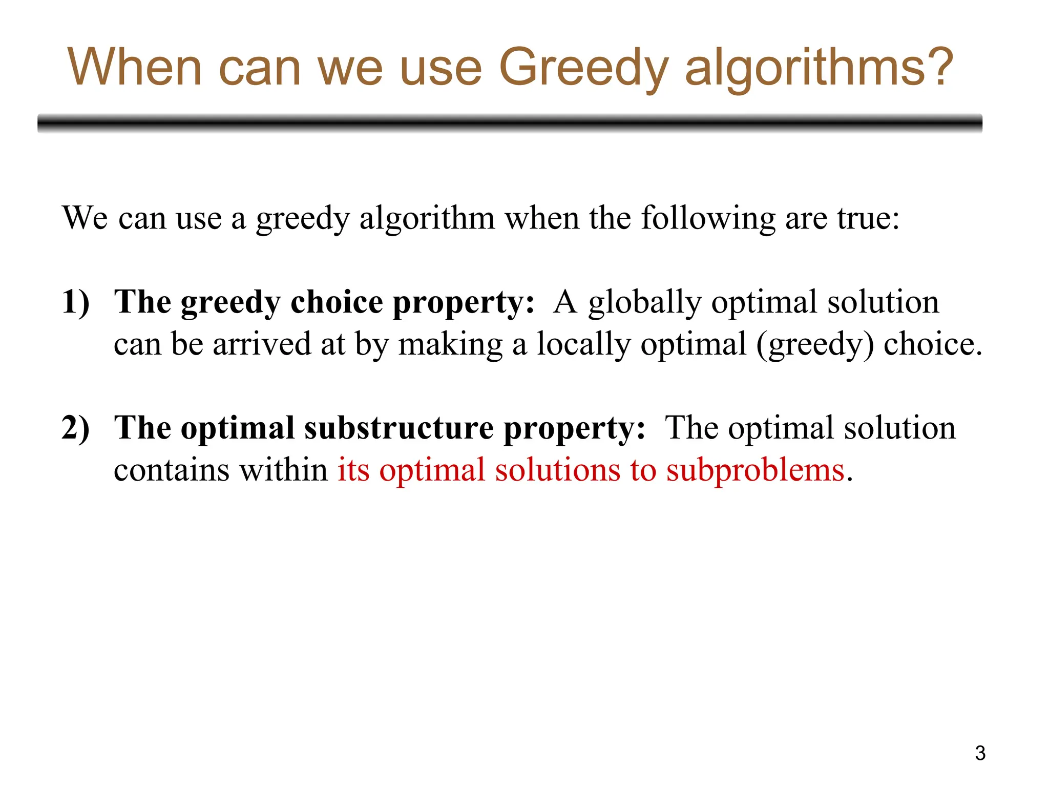
When can we use Greedy algorithms?
We can use a greedy algorithm when the following are true:
1) The greedy choice property: A globally optimal solution
can be arrived at by making a locally optimal (greedy) choice.
2) The optimal substructure property: The optimal solution
contains within its optimal solutions to subproblems.

4
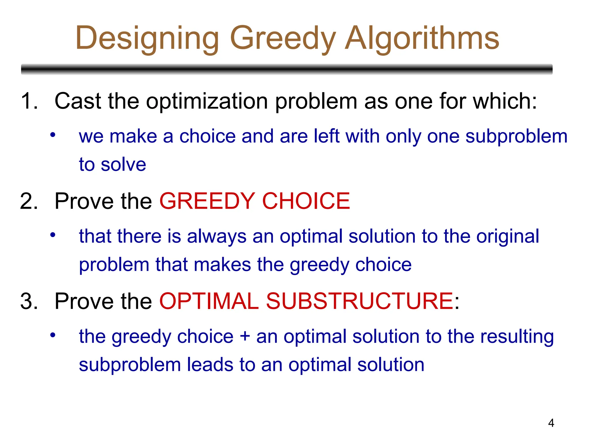
Designing Greedy Algorithms
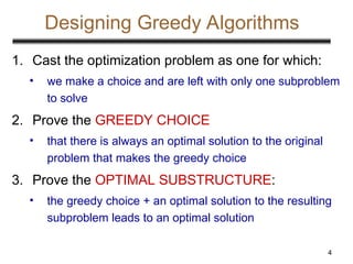
1. Cast the optimization problem as one for which:
• we make a choice and are left with only one subproblem
to solve
2. Prove the GREEDY CHOICE
• that there is always an optimal solution to the original
problem that makes the greedy choice
3. Prove the OPTIMAL SUBSTRUCTURE:
• the greedy choice + an optimal solution to the resulting
subproblem leads to an optimal solution

Greedy Algorithms
Part -1 : Greedy Coin Changing Algorithm

Objective
7
Pay out a given sum S with the smallest
number of coins possible.

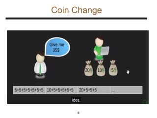
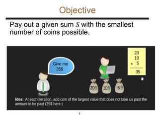
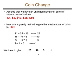
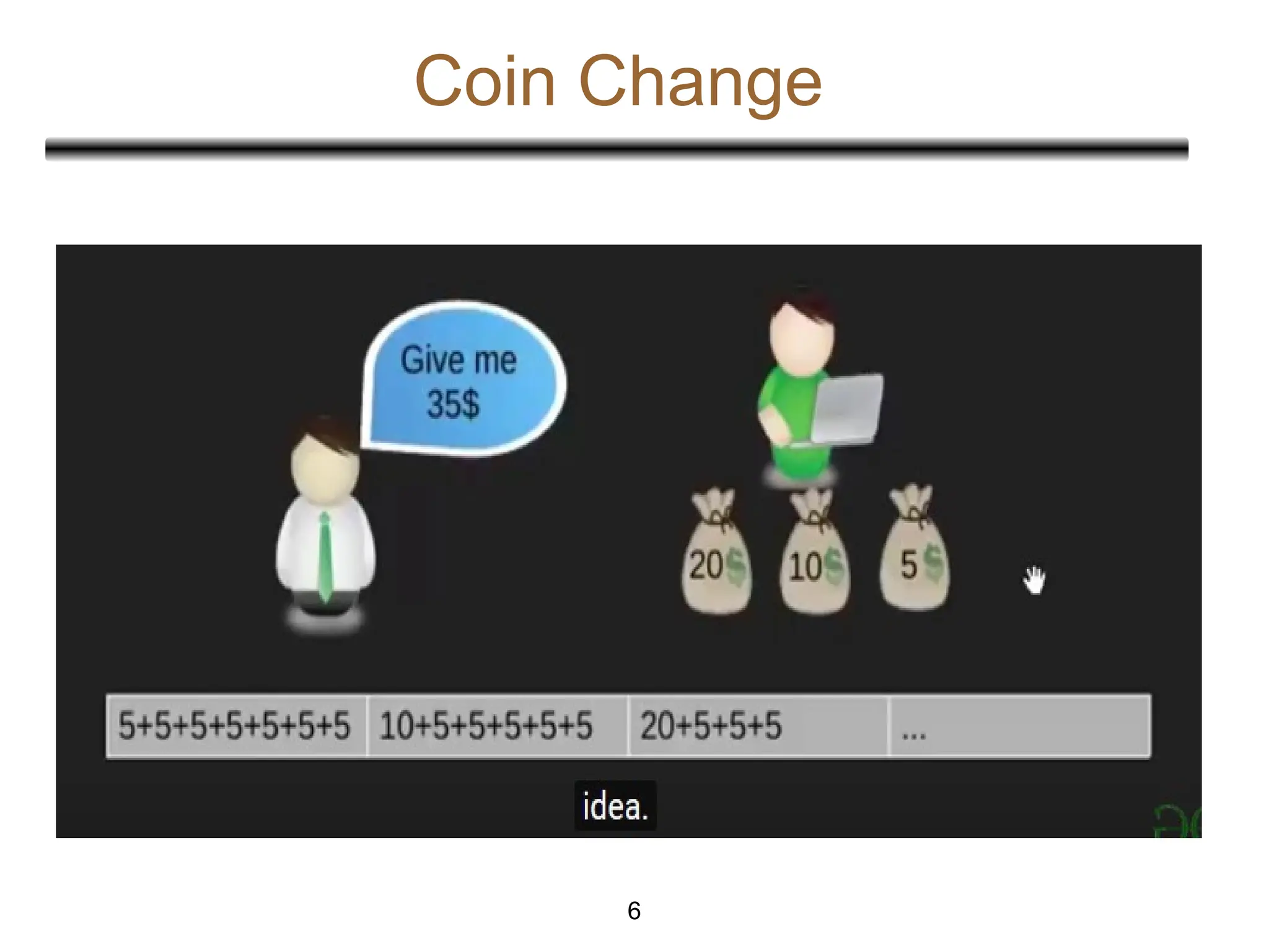
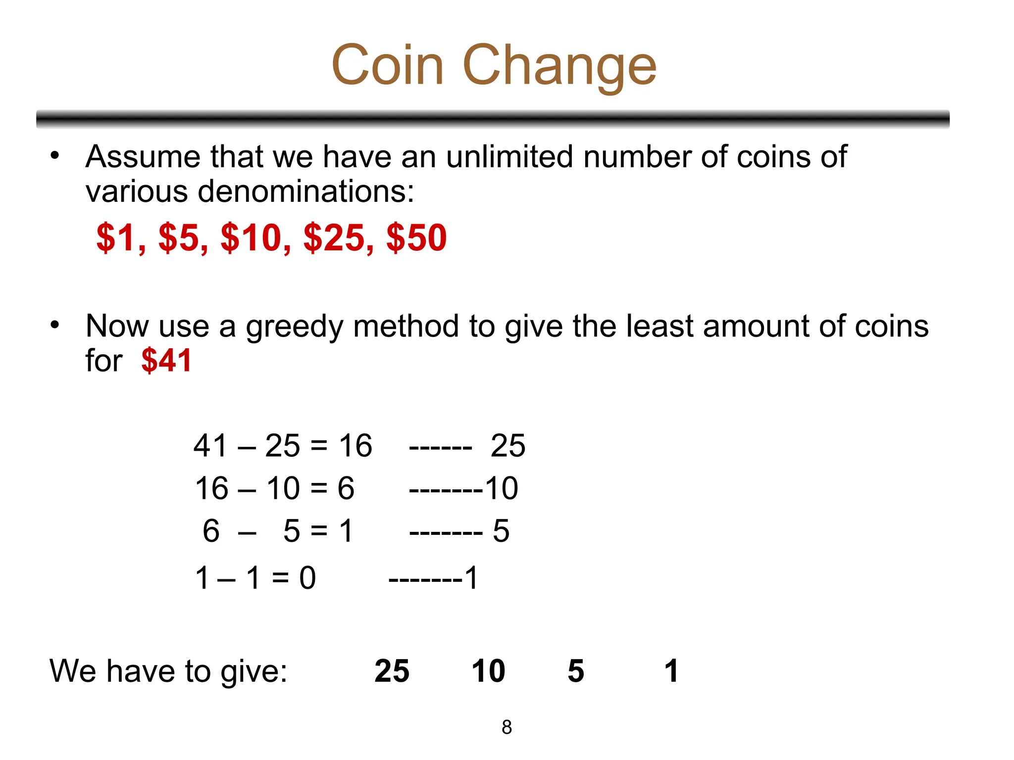
Coin Change
• Assume that we have an unlimited number of coins of
various denominations:
$1, $5, $10, $25, $50
• Now use a greedy method to give the least amount of coins
for $41
41 – 25 = 16 ------ 25
16 – 10 = 6 -------10
6 – 5 = 1 ------- 5
1 – 1 = 0 -------1
We have to give: 25 10 5 1
8

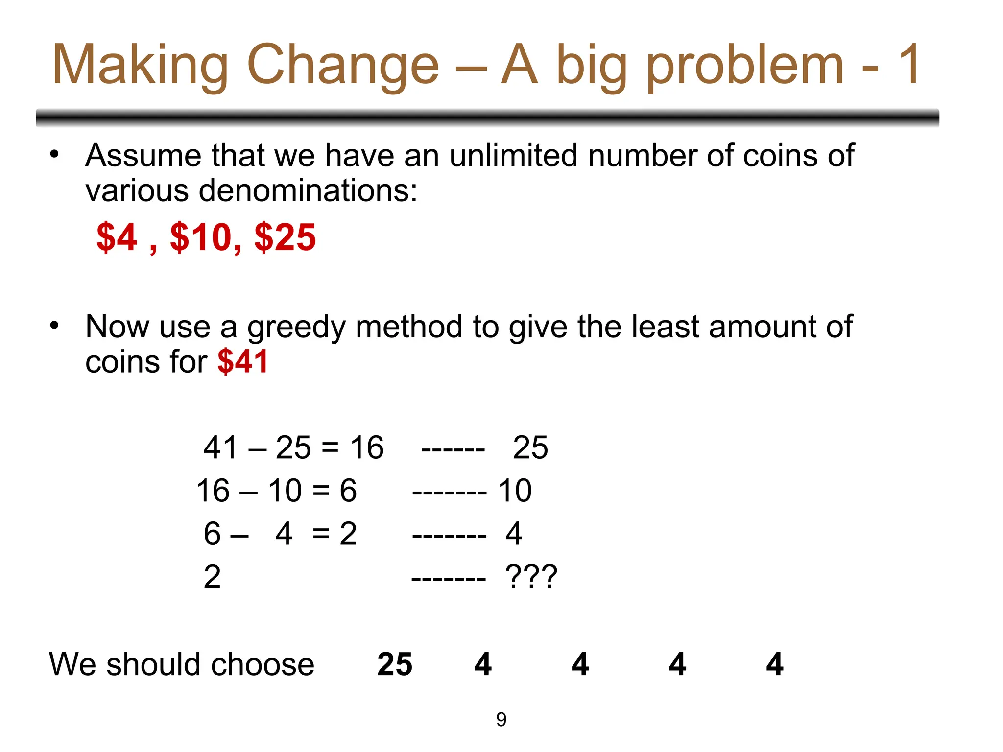
Making Change – A big problem - 1
• Assume that we have an unlimited number of coins of
various denominations:
$4 , $10, $25
• Now use a greedy method to give the least amount of
coins for $41
41 – 25 = 16 ------ 25
16 – 10 = 6 ------- 10
6 – 4 = 2 ------- 4
2 ------- ???
We should choose 25 4 4 4 4
9

10
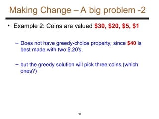
Making Change – A big problem -2
• Example 2: Coins are valued $30, $20, $5, $1
– Does not have greedy-choice property, since $40 is
best made with two $.20’s,
– but the greedy solution will pick three coins (which
ones?)

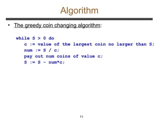
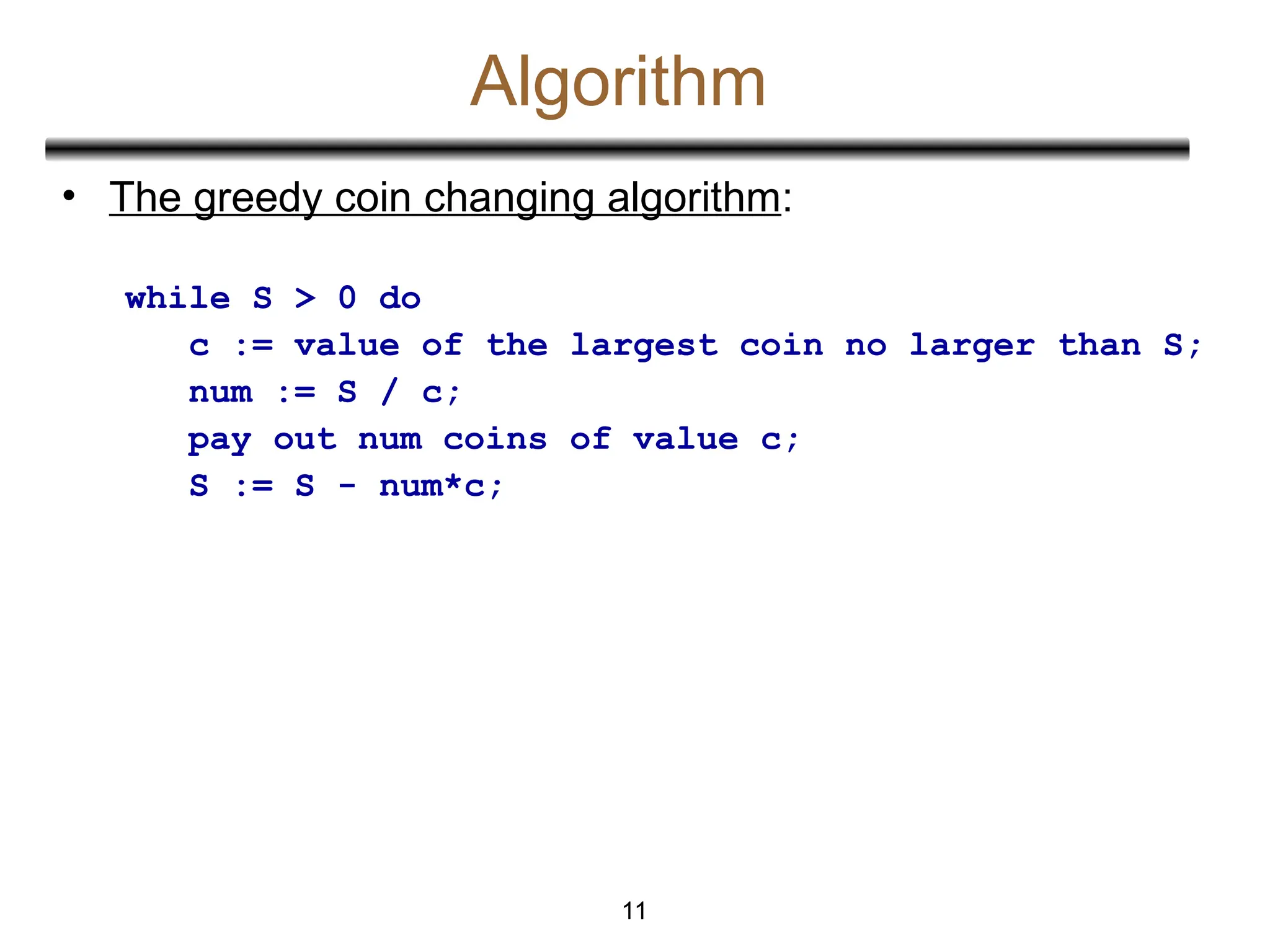
Algorithm
• The greedy coin changing algorithm:
while S > 0 do
c := value of the largest coin no larger than S;
num := S / c;
pay out num coins of value c;
S := S - num*c;
11

Greedy Algorithms
Part -2 : The Fractional Knapsack Problem

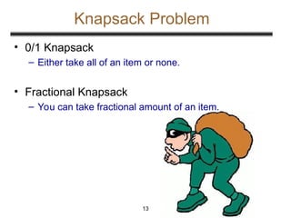
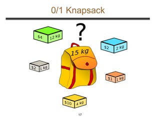
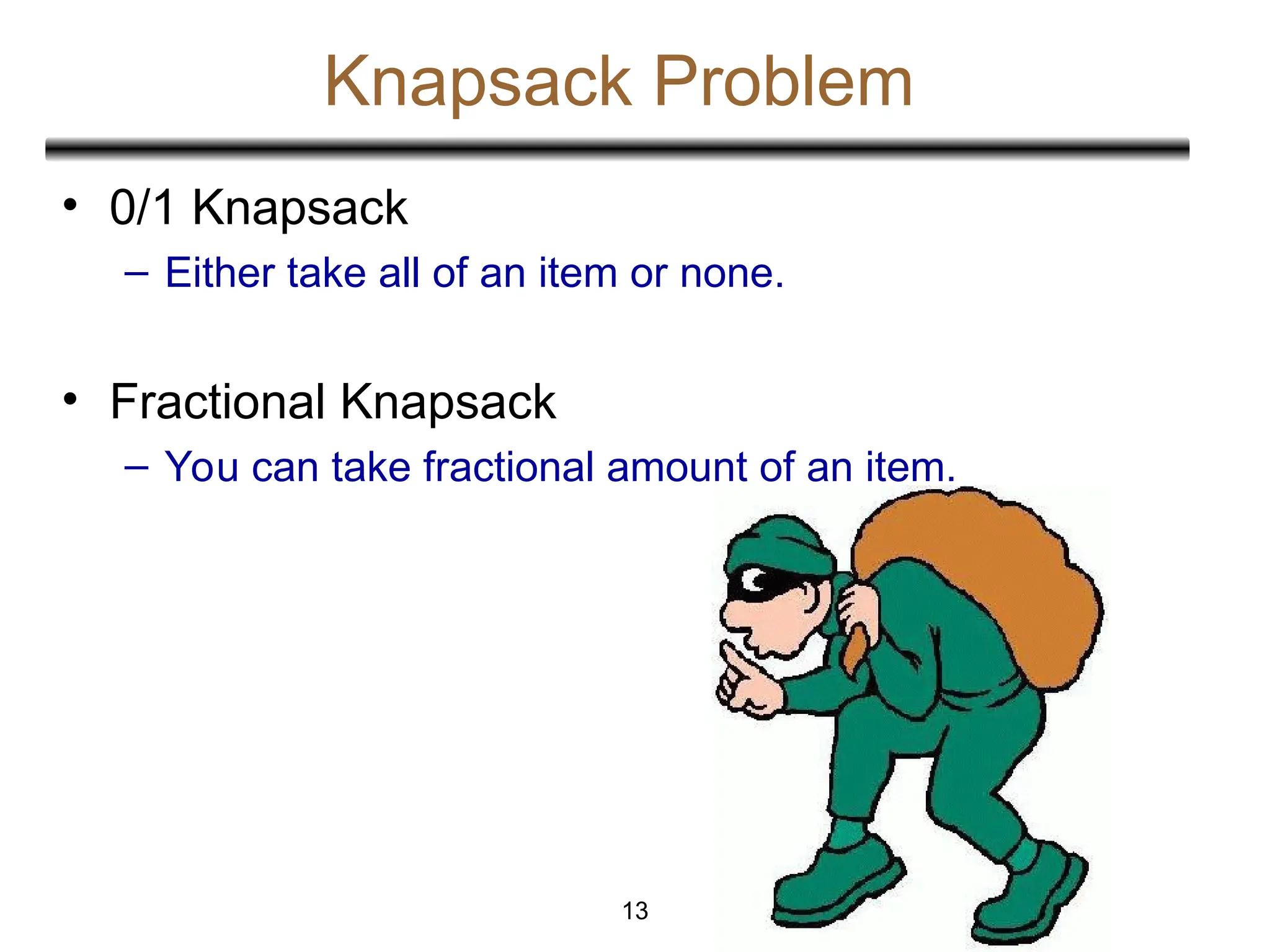
Knapsack Problem
• 0/1 Knapsack
– Either take all of an item or none.
• Fractional Knapsack
– You can take fractional amount of an item.
13

14
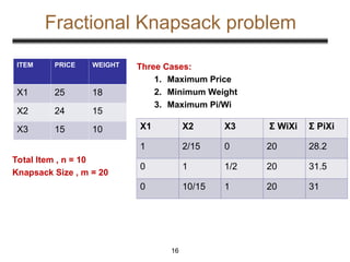
Concept of Knapsack Problem
• A Set of Items are given where,
– No of Items = n [X1, X2, X3, ….. Xn]
– Weight of Xi = Wi
– Profit of Xi = Pi
– Knapsack Size = m
• Goal:
– Maximize the Profit ΣPiXi
within ΣWiXi <= m

Fractional Knapsack problem
ITEM PRICE WEIGHT
X1 25 18
X2 24 15
X3 15 10
16
Total Item , n = 10
Knapsack Size , m = 20
X1 X2 X3 Σ WiXi Σ PiXi
1 2/15 0 20 28.2
0 1 1/2 20 31.5
0 10/15 1 20 31
Three Cases:
1. Maximum Price
2. Minimum Weight
3. Maximum Pi/Wi

18
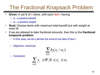
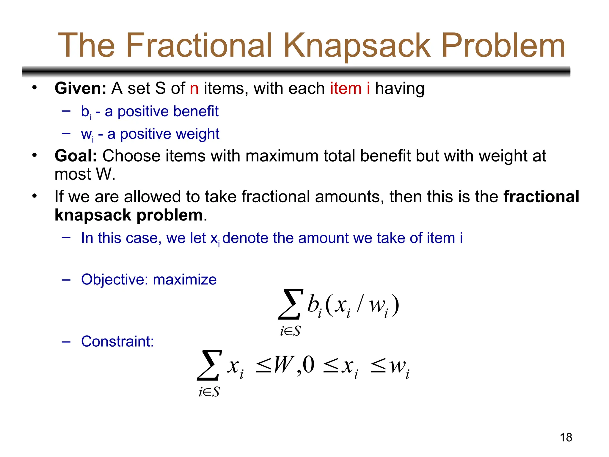
The Fractional Knapsack Problem
• Given: A set S of n items, with each item i having
– bi - a positive benefit
– wi - a positive weight
• Goal: Choose items with maximum total benefit but with weight at
most W.
• If we are allowed to take fractional amounts, then this is the fractional
knapsack problem.
– In this case, we let xi denote the amount we take of item i
– Objective: maximize
– Constraint:

S
i
i
i
i w
x
b )
/
(
i
i
S
i
i w
x
W
x 




0
,

19
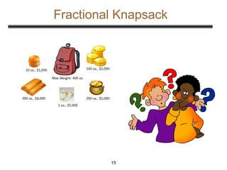
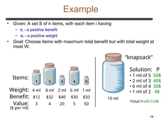
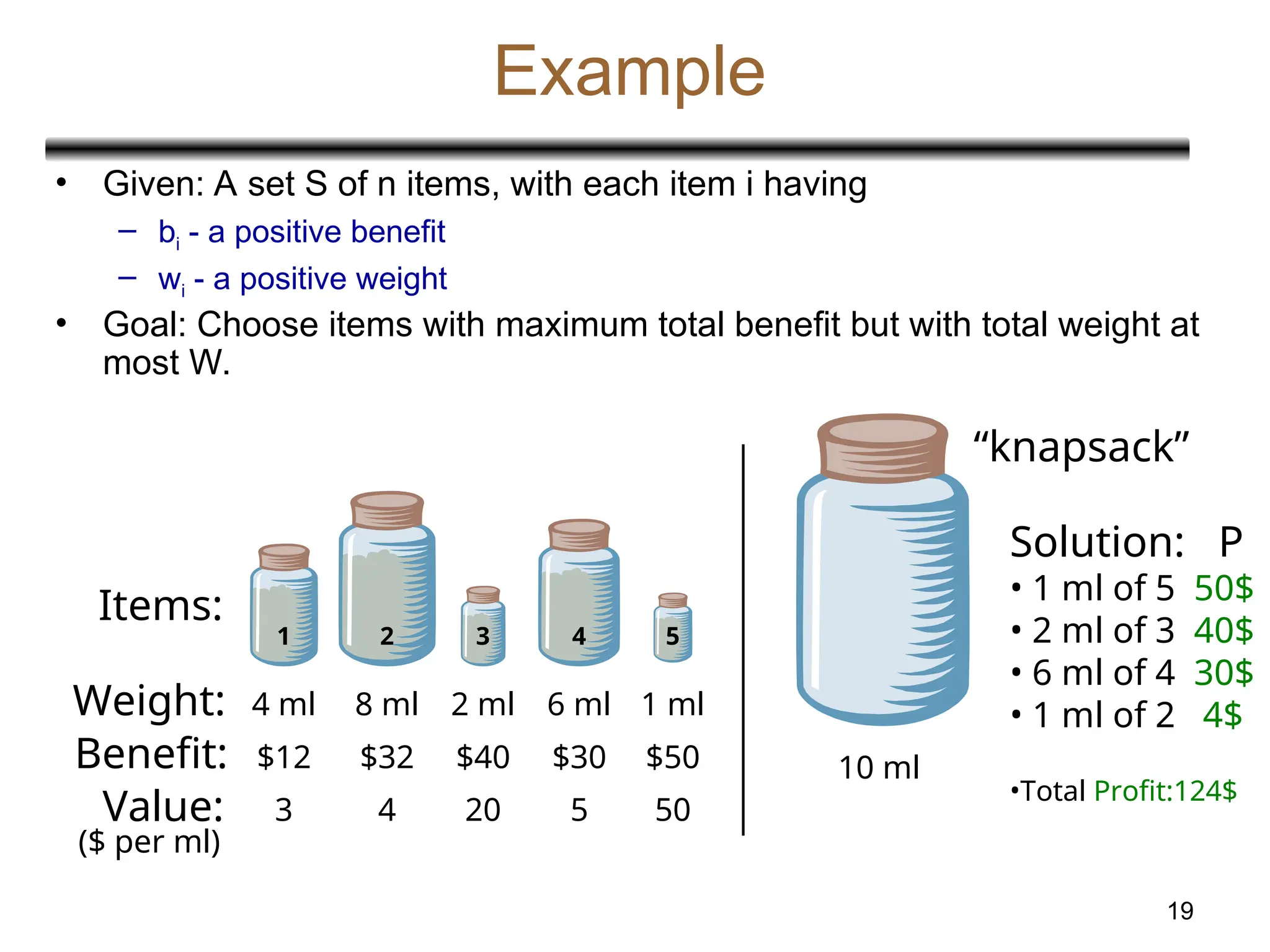
Example
• Given: A set S of n items, with each item i having
– bi - a positive benefit
– wi - a positive weight
• Goal: Choose items with maximum total benefit but with total weight at
most W.
Weight:
Benefit:
1 2 3 4 5
4 ml 8 ml 2 ml 6 ml 1 ml
$12 $32 $40 $30 $50
Items:
Value: 3
($ per ml)
4 20 5 50
10 ml
Solution: P
• 1 ml of 5 50$
• 2 ml of 3 40$
• 6 ml of 4 30$
• 1 ml of 2 4$
•Total Profit:124$
“knapsack”

20
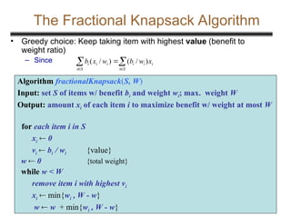
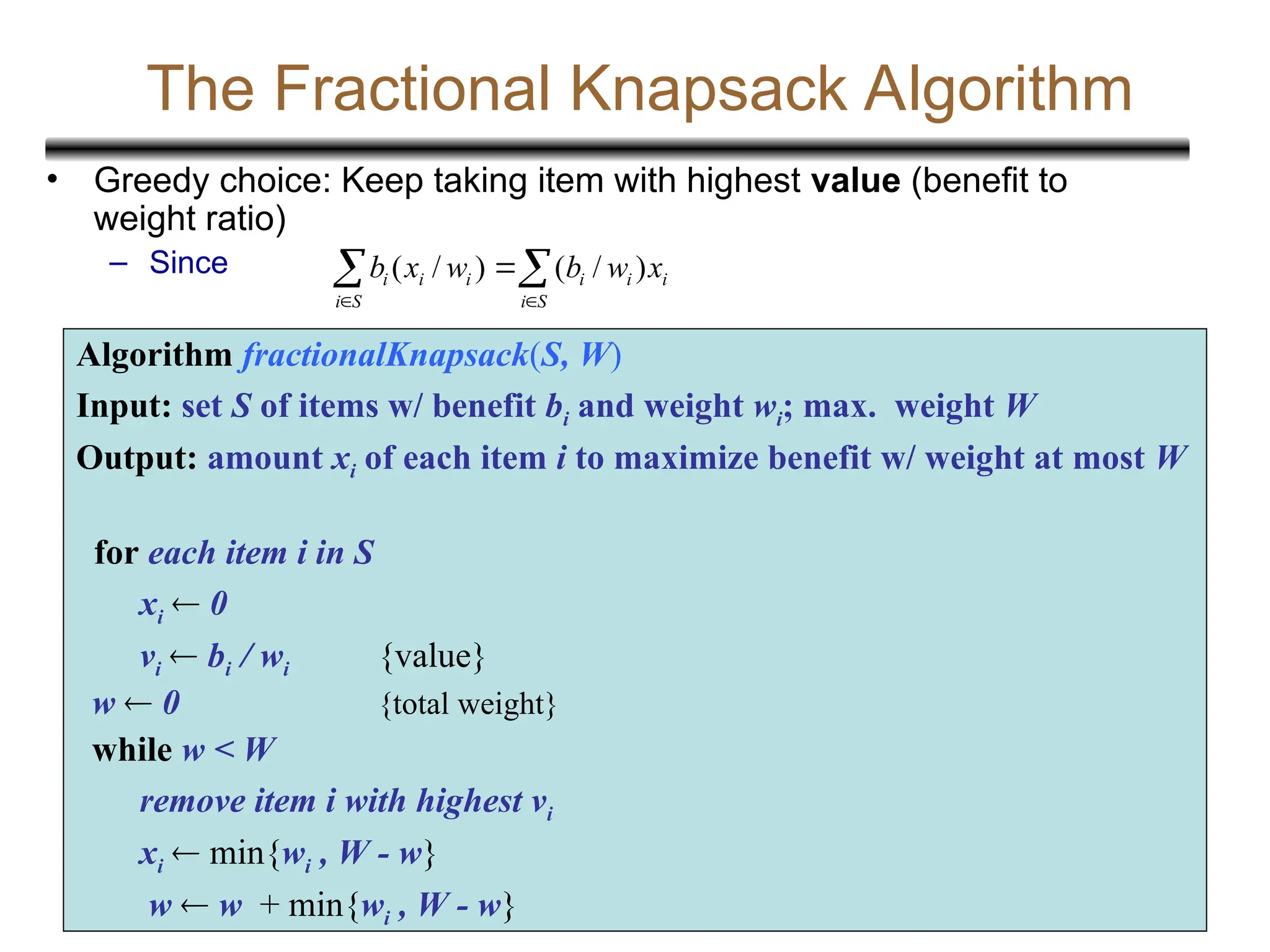
The Fractional Knapsack Algorithm
• Greedy choice: Keep taking item with highest value (benefit to
weight ratio)
– Since
Algorithm fractionalKnapsack(S, W)
Input: set S of items w/ benefit bi and weight wi; max. weight W
Output: amount xi of each item i to maximize benefit w/ weight at most W
for each item i in S
xi  0
vi  bi / wi {value}
w  0 {total weight}
while w < W
remove item i with highest vi
xi  min{wi , W - w}
w  w + min{wi , W - w}

 


S
i
i
i
i
S
i
i
i
i x
w
b
w
x
b )
/
(
)
/
(

21
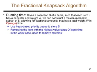
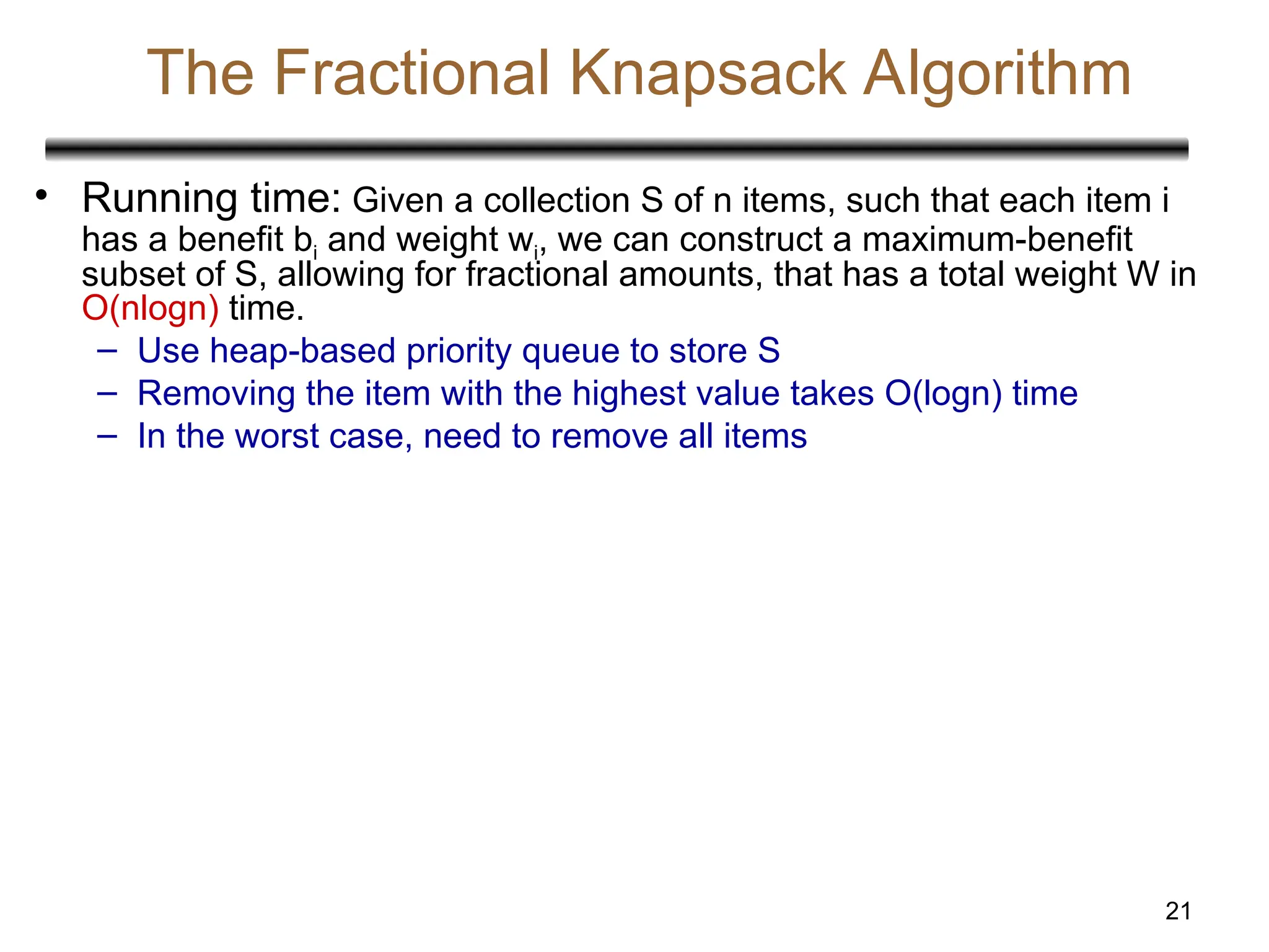
The Fractional Knapsack Algorithm
• Running time: Given a collection S of n items, such that each item i
has a benefit bi and weight wi, we can construct a maximum-benefit
subset of S, allowing for fractional amounts, that has a total weight W in
O(nlogn) time.
– Use heap-based priority queue to store S
– Removing the item with the highest value takes O(logn) time
– In the worst case, need to remove all items

Greedy Algorithms
Part -3 : Huffman Codes

23
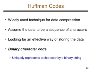
Huffman Codes
• Widely used technique for data compression
• Assume the data to be a sequence of characters
• Looking for an effective way of storing the data
• Binary character code
– Uniquely represents a character by a binary string

24
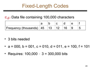
Fixed-Length Codes
E.g.: Data file containing 100,000 characters
• 3 bits needed
• a = 000, b = 001, c = 010, d = 011, e = 100, f = 101
• Requires: 100,000  3 = 300,000 bits
a b c d e f
Frequency (thousands) 45 13 12 16 9 5

25
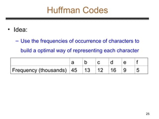
Huffman Codes
• Idea:
– Use the frequencies of occurrence of characters to
build a optimal way of representing each character
a b c d e f

26
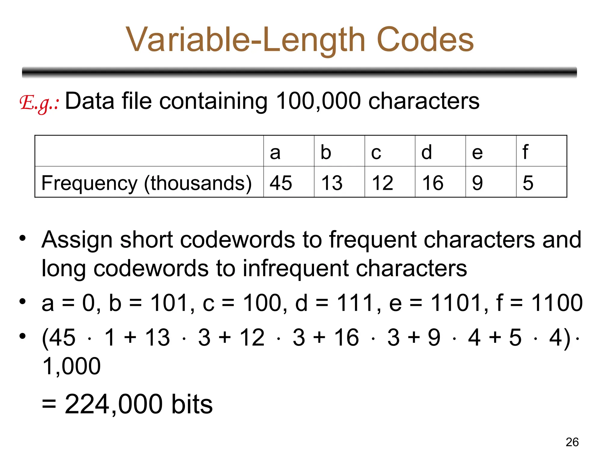
Variable-Length Codes
E.g.: Data file containing 100,000 characters
• Assign short codewords to frequent characters and
long codewords to infrequent characters
• a = 0, b = 101, c = 100, d = 111, e = 1101, f = 1100
• (45  1 + 13  3 + 12  3 + 16  3 + 9  4 + 5  4)
1,000
= 224,000 bits
a b c d e f

27
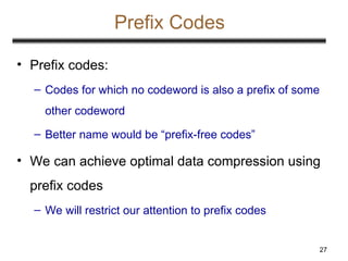
Prefix Codes
• Prefix codes:
– Codes for which no codeword is also a prefix of some
other codeword
– Better name would be “prefix-free codes”
• We can achieve optimal data compression using
prefix codes
– We will restrict our attention to prefix codes

28
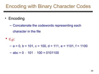
Encoding with Binary Character Codes
• Encoding
– Concatenate the codewords representing each
character in the file
• E.g.:
– a = 0, b = 101, c = 100, d = 111, e = 1101, f = 1100
– abc = 0  101  100 = 0101100

29
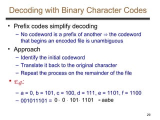
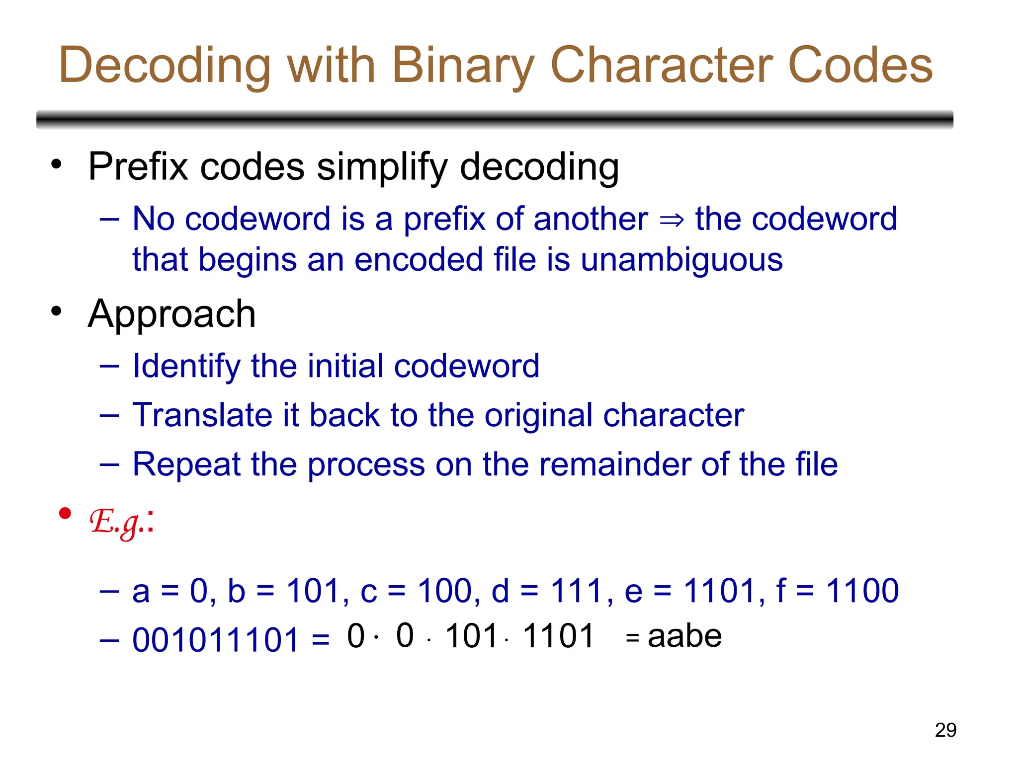
Decoding with Binary Character Codes
• Prefix codes simplify decoding
– No codeword is a prefix of another  the codeword
that begins an encoded file is unambiguous
• Approach
– Identify the initial codeword
– Translate it back to the original character
– Repeat the process on the remainder of the file
• E.g.:
– a = 0, b = 101, c = 100, d = 111, e = 1101, f = 1100
– 001011101 = 0 0  101 1101 = aabe

30
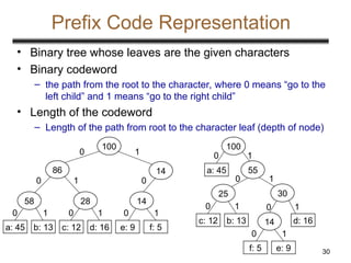
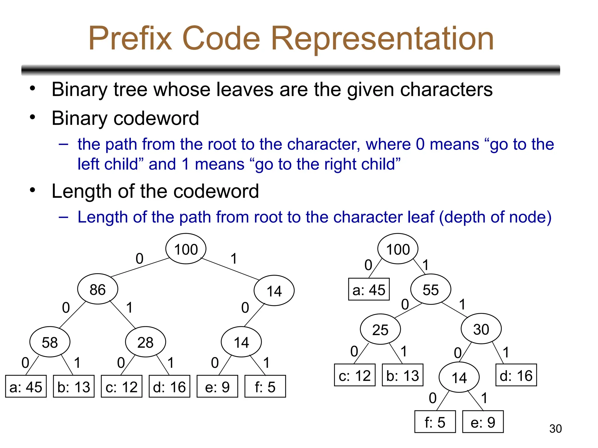
Prefix Code Representation
• Binary tree whose leaves are the given characters
• Binary codeword
– the path from the root to the character, where 0 means “go to the
left child” and 1 means “go to the right child”
• Length of the codeword
– Length of the path from root to the character leaf (depth of node)
100
86 14
58 28 14
a: 45 b: 13 c: 12 d: 16 e: 9 f: 5
0
0
0
1
1 1
1
1
0
0 0
100
a: 45
0
55
1
25 30
0 1
c: 12 b: 13
1
0
14
f: 5 e: 9
1
0
d: 16
1
0

31
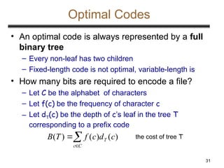
Optimal Codes
• An optimal code is always represented by a full
binary tree
– Every non-leaf has two children
– Fixed-length code is not optimal, variable-length is
• How many bits are required to encode a file?
– Let C be the alphabet of characters
– Let f(c) be the frequency of character c
– Let dT(c) be the depth of c’s leaf in the tree T
corresponding to a prefix code



C
c
T c
d
c
f
T
B )
(
)
(
)
( the cost of tree T

32
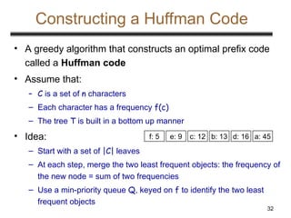
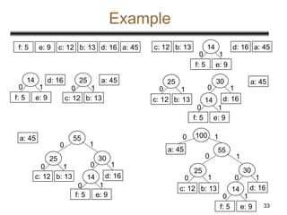
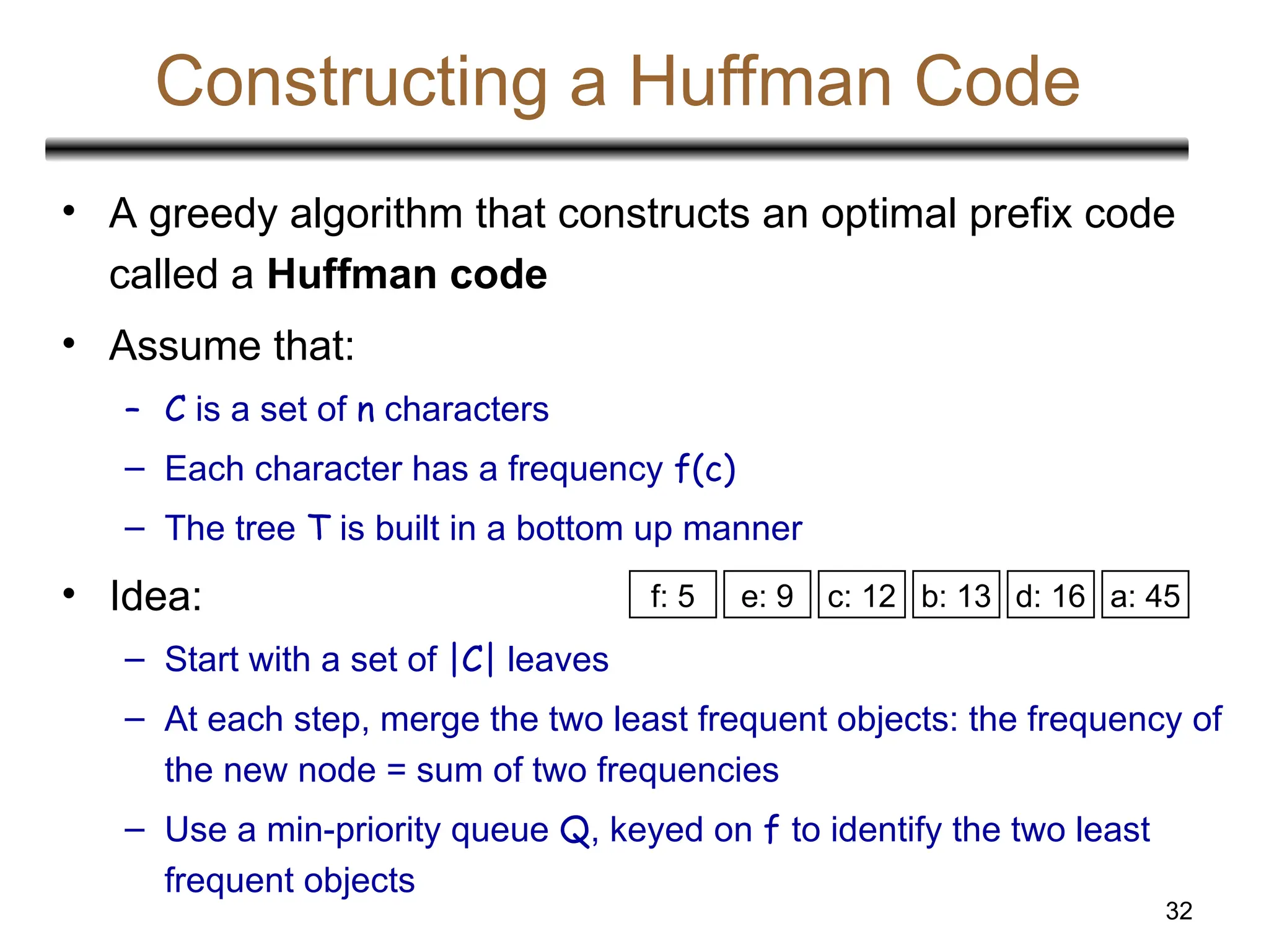
Constructing a Huffman Code
• A greedy algorithm that constructs an optimal prefix code
called a Huffman code
• Assume that:
– C is a set of n characters
– Each character has a frequency f(c)
– The tree T is built in a bottom up manner
• Idea:
– Start with a set of |C| leaves
– At each step, merge the two least frequent objects: the frequency of
the new node = sum of two frequencies
– Use a min-priority queue Q, keyed on f to identify the two least
frequent objects
a: 45
c: 12 b: 13
f: 5 e: 9 d: 16

33
Example
a: 45
c: 12 b: 13
f: 5 e: 9 d: 16 a: 45
c: 12 b: 13 d: 16
14
f: 5 e: 9
0 1
d: 16
c: 12 b: 13
25 a: 45
f: 5 e: 9
14
0 0
1 1
f: 5 e: 9
14
c: 12 b: 13
25
d: 16
30 a: 45
0 0
0
1 1
1
a: 45
f: 5 e: 9
14
c: 12 b: 13
25
d: 16
30
55
0
0 0
0
1
1
1
1
f: 5 e: 9
14
c: 12 b: 13
25
d: 16
30
55
a: 45
100
0
0
0 0
0
1
1
1
1
1

34
Building a Huffman Code
Alg.: HUFFMAN(C)
1. n  C 
2. Q  C
3. for i  1 to n – 1
4. do allocate a new node z
5. left[z]  x  EXTRACT-MIN(Q)
6. right[z]  y  EXTRACT-MIN(Q)
7. f[z]  f[x] + f[y]
8. INSERT (Q, z)
9. return EXTRACT-MIN(Q)
O(n)
O(nlgn)
Running time: O(nlgn)

Greedy Algorithms
Part -4 : Bin Packing Problem

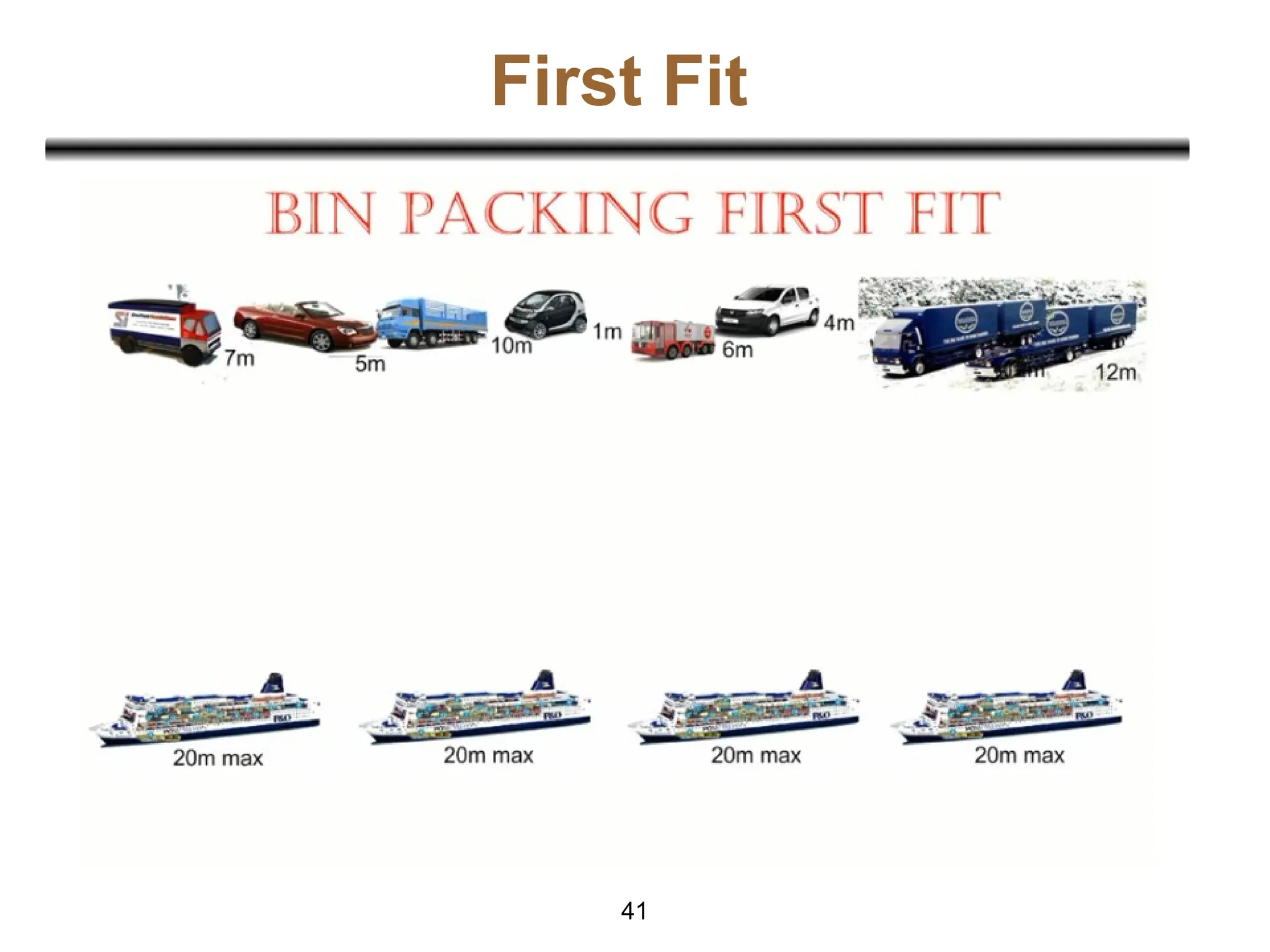
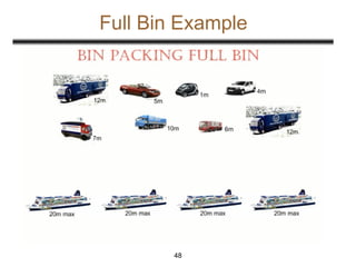
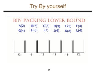
Bin Packing
37
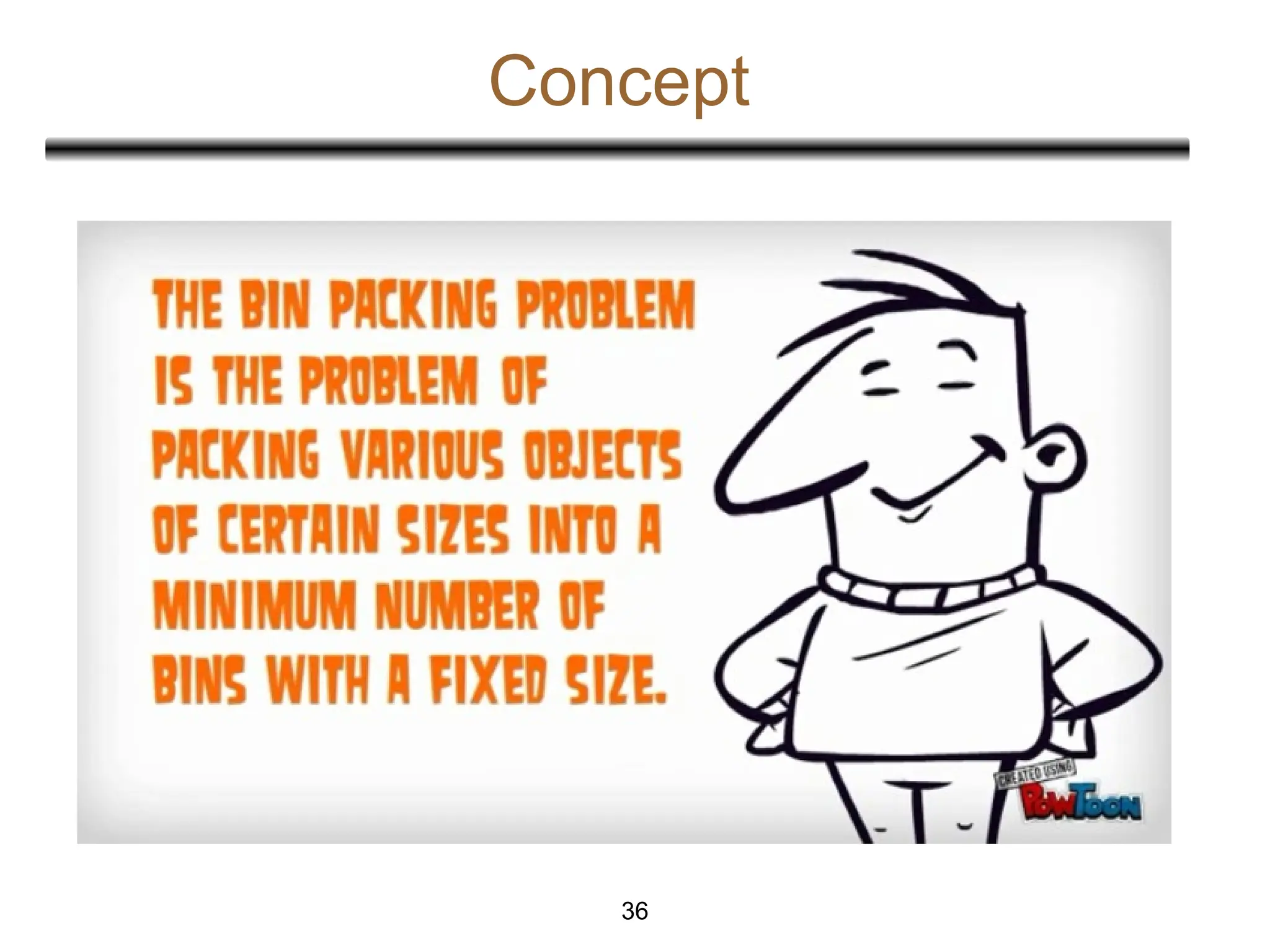
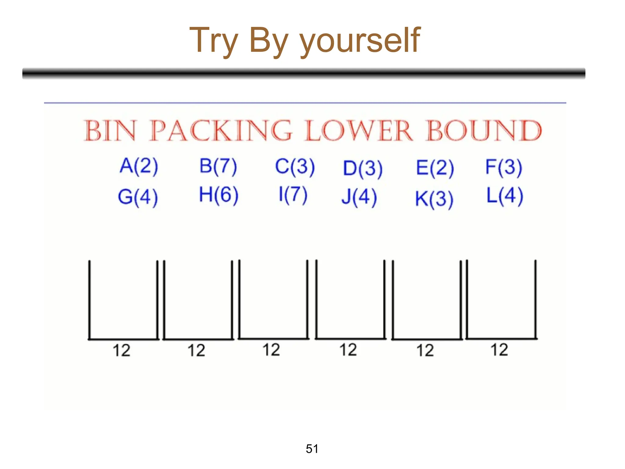
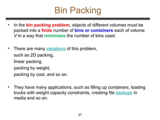
• In the bin packing problem, objects of different volumes must be
packed into a finite number of bins or containers each of volume
V in a way that minimizes the number of bins used.
• There are many variations of this problem,
such as 2D packing,
linear packing,
packing by weight,
packing by cost, and so on.
• They have many applications, such as filling up containers, loading
trucks with weight capacity constraints, creating file backups in
media and so on.

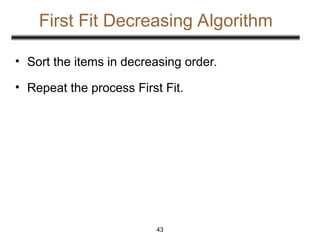
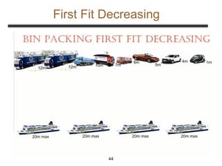
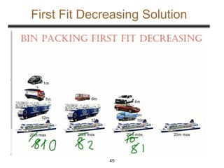
Ways of Solution
• First Fit Algorithm
• First Fit Decreasing Algorithm
• Full Bin Algorithm
• Other Algorithms
38

Find The Lower Bound
39
Total size = 12 + 12 + 7 + 6
+ 10 + 4 + 5 + 1 = 57
Bin Size = 20
Lower Bound = 57/20
= 2.85 = 3

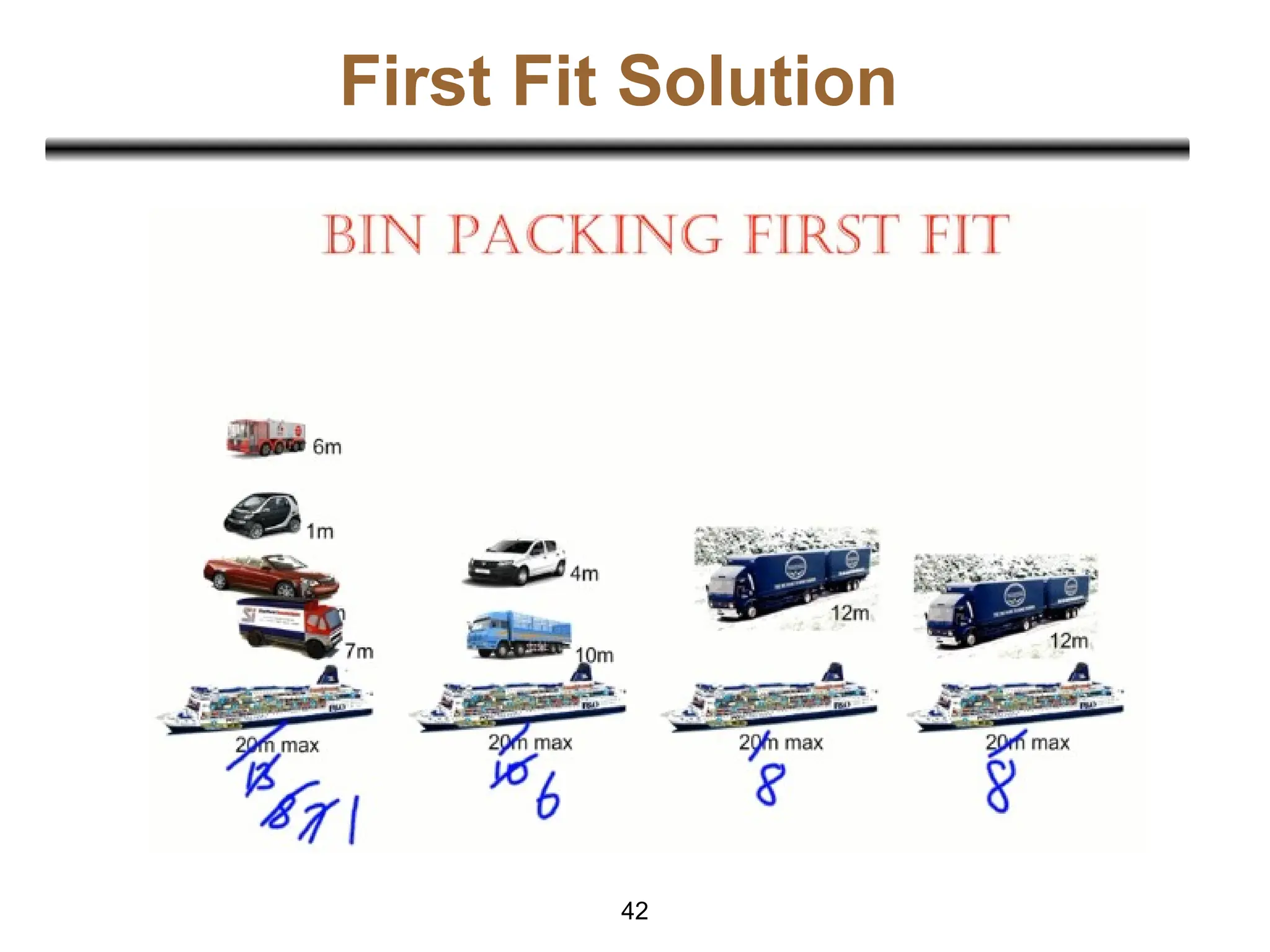
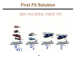
First Fit Algorithm
• This is a very straightforward greedy
approximation algorithm.
• The algorithm processes the items in arbitrary
order.
• For each item, it attempts to place the item in the
first bin that can accommodate the item. If no bin
is found, it opens a new bin and puts the item
within the new bin.
40

First Fit Decreasing Algorithm
• Sort the items in decreasing order.
• Repeat the process First Fit.
43

First Fit Decreasing Solution
45

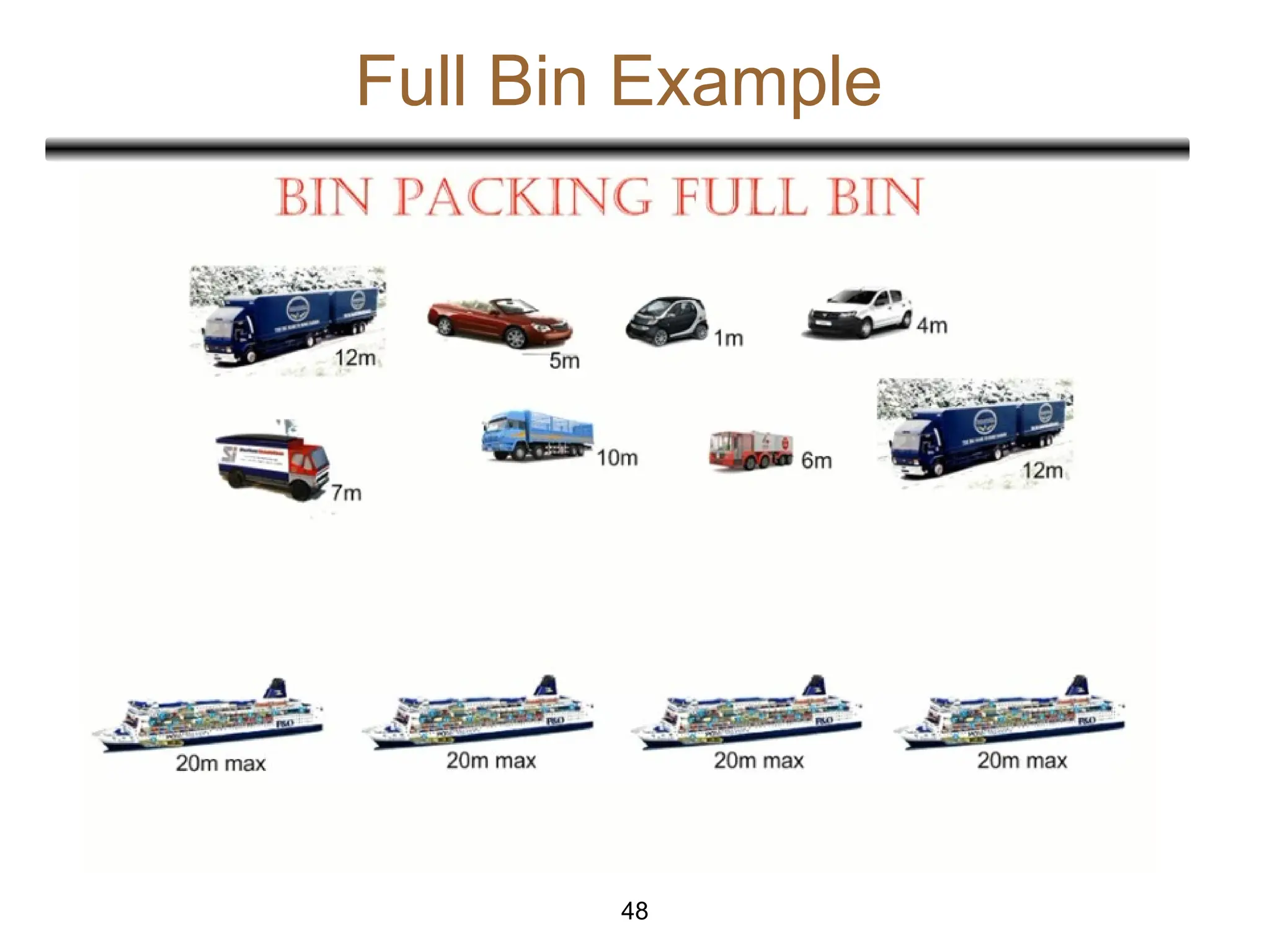
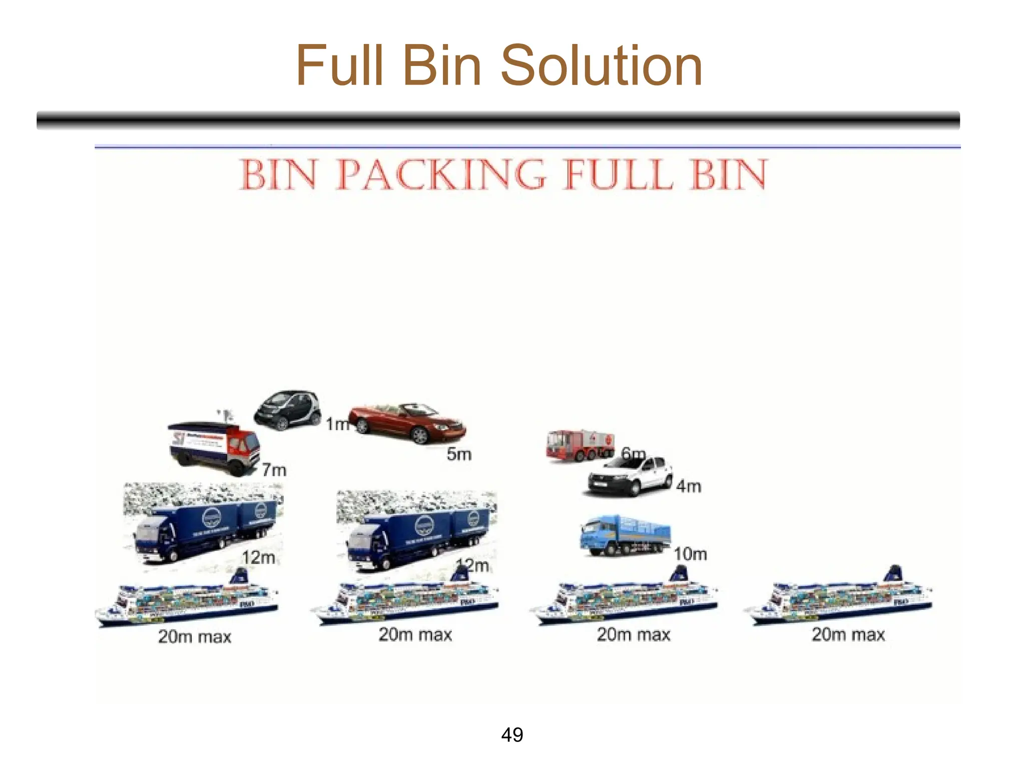
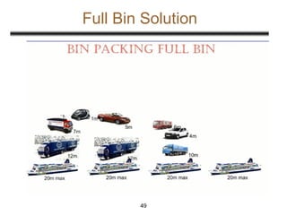
Full Bin Algorithm
• The full bin packing algorithm is more likely to
produce an optimal solution – using the least
possible number of bins – than the first fit
decreasing and first fit algorithms. It works by
matching object so as to fill as many bins as
possible.
46

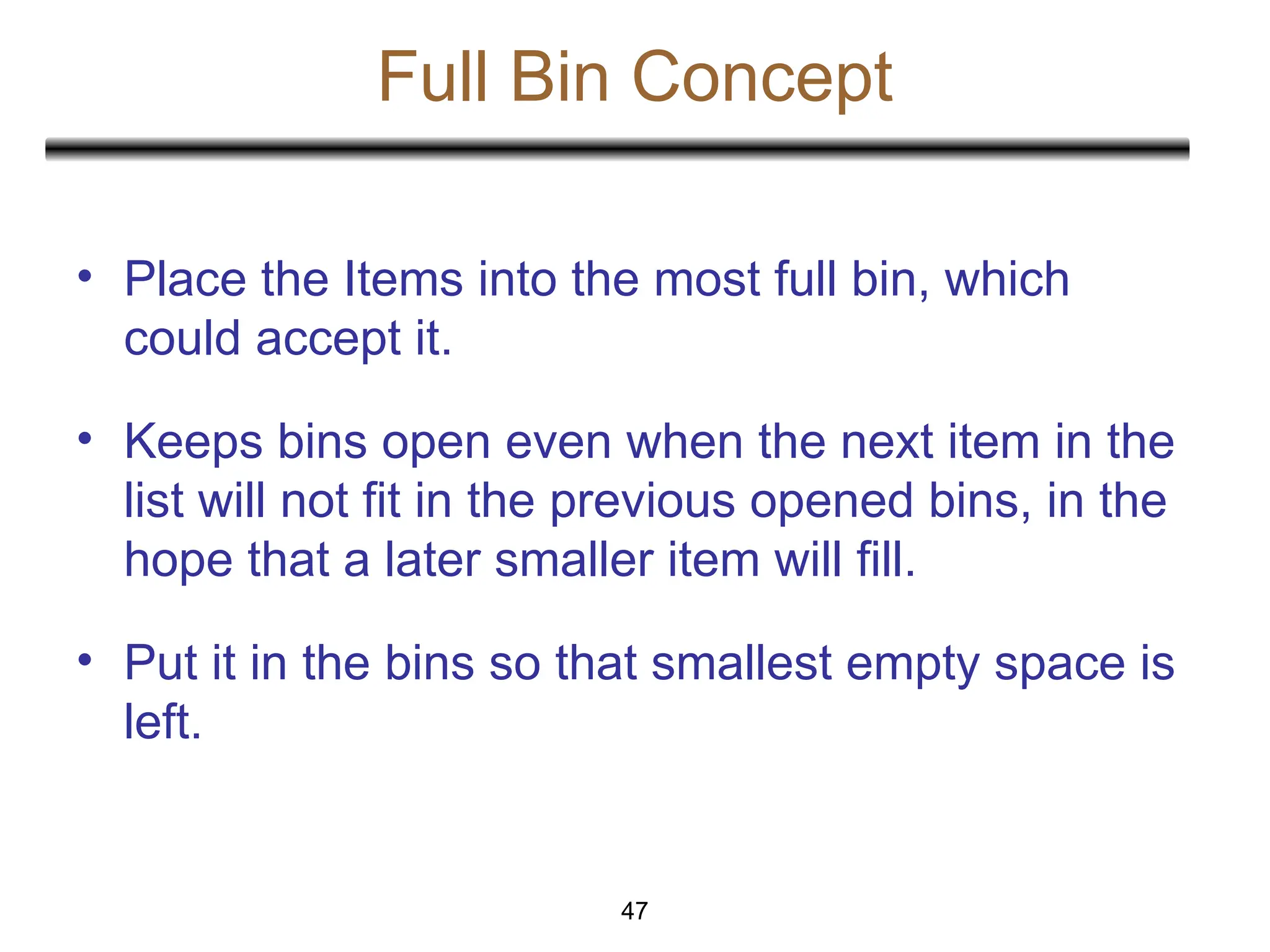
Full Bin Concept
47
• Place the Items into the most full bin, which
could accept it.
• Keeps bins open even when the next item in the
list will not fit in the previous opened bins, in the
hope that a later smaller item will fill.
• Put it in the bins so that smallest empty space is
left.

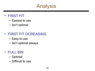
Analysis
50
• FIRST FIT
– Easiest to use
– Isn’t optimal
• FIRST FIT DCREASING
– Easy to use
– Isn’t optimal always
• FULL BIN
– Optimal
– Difficult to use

Drawbacks of Greedy Methods
Does not always find the optimal solution for
some problems.
52

Presentation on Greedy Algorithm process.ppt

More Related Content

Similar to Presentation on Greedy Algorithm process.ppt

Recently uploaded

Presentation on Greedy Algorithm process.ppt