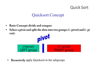
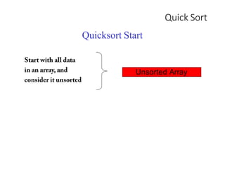
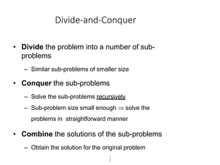
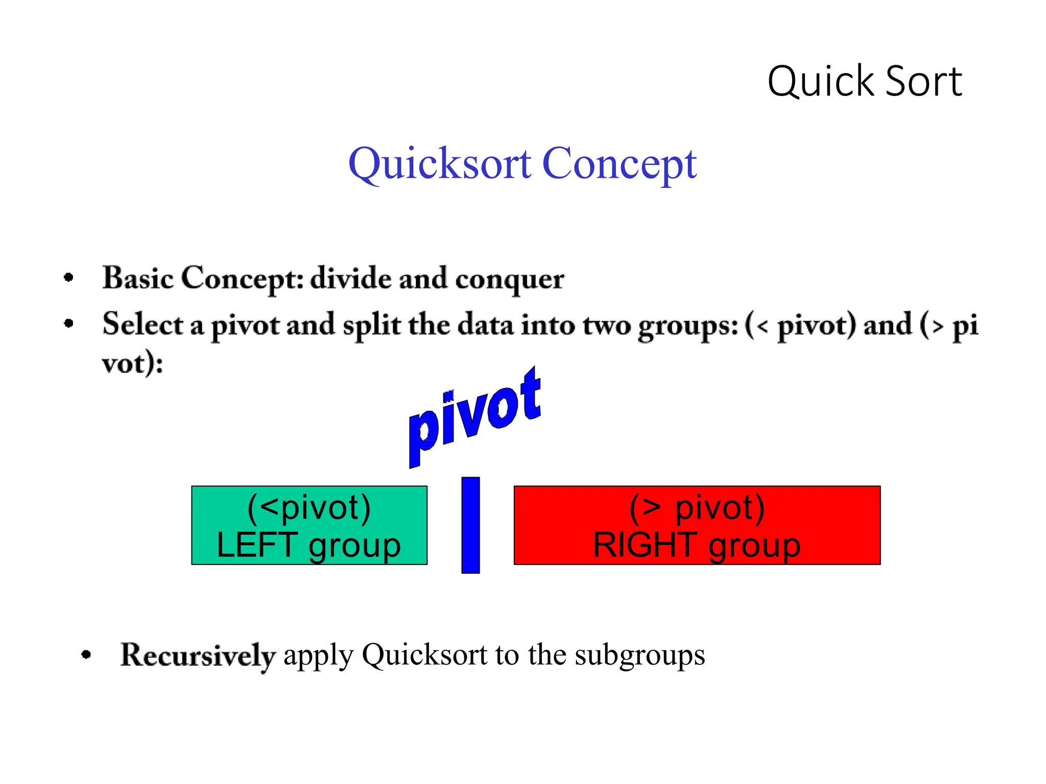
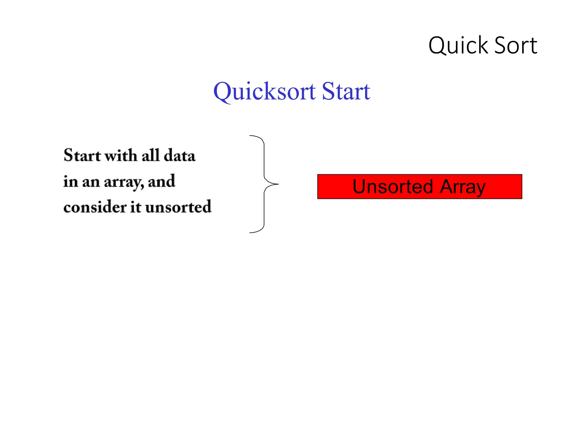
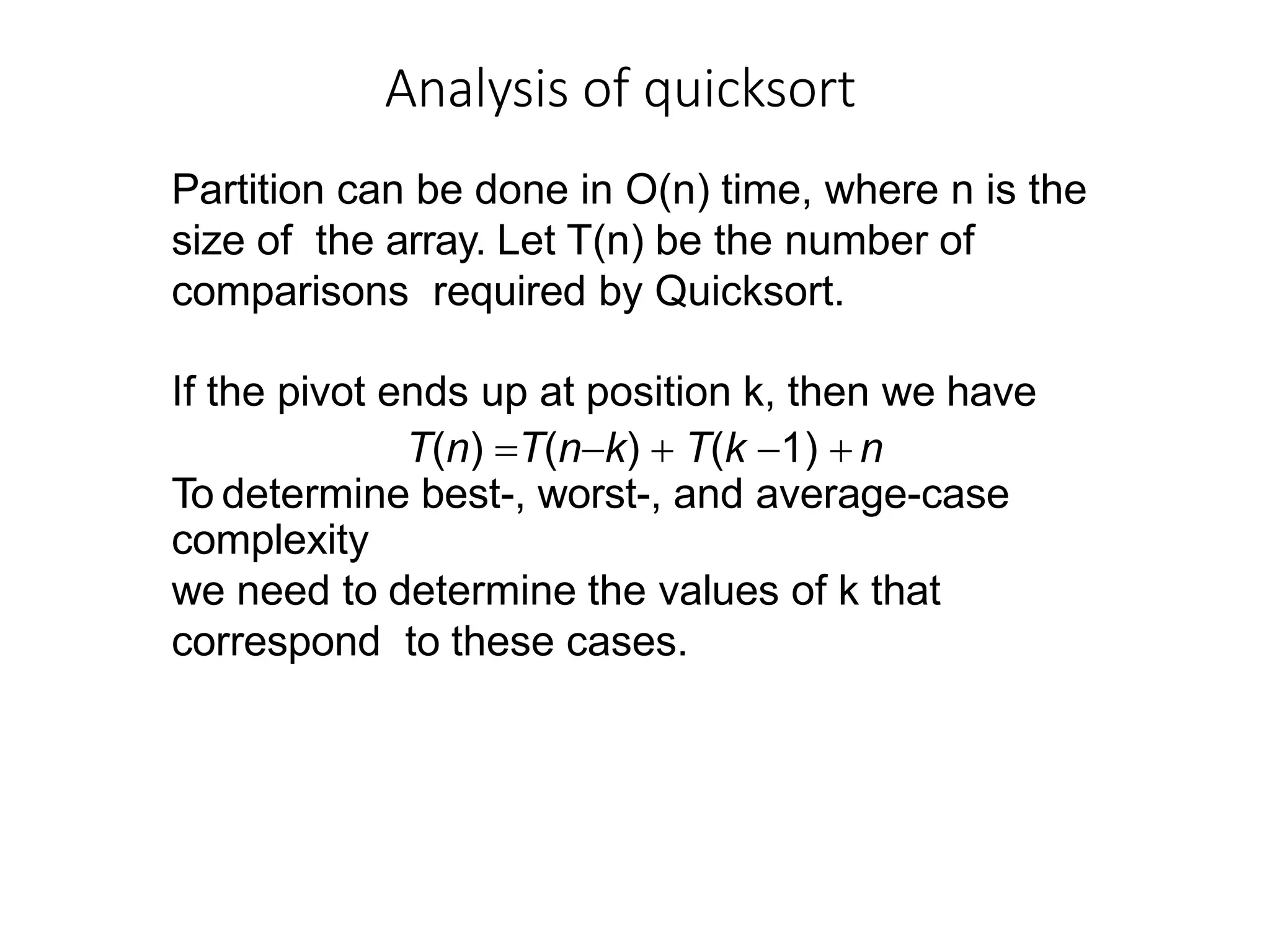
Quicksort is a divide and conquer algorithm that works by partitioning an array around a pivot value and recursively sorting the subarrays. It has the following steps:
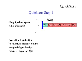
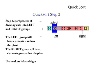
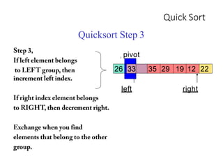
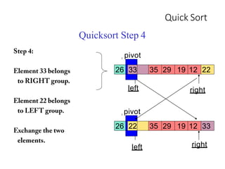
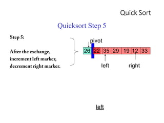
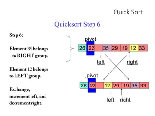
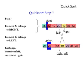
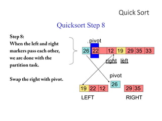
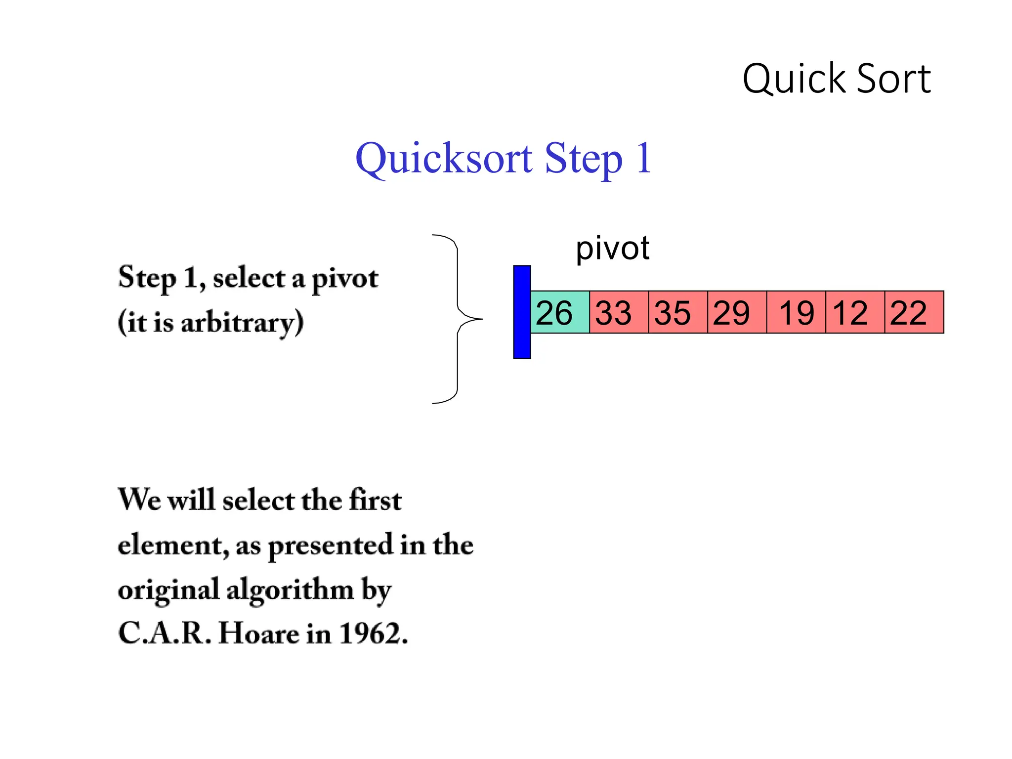
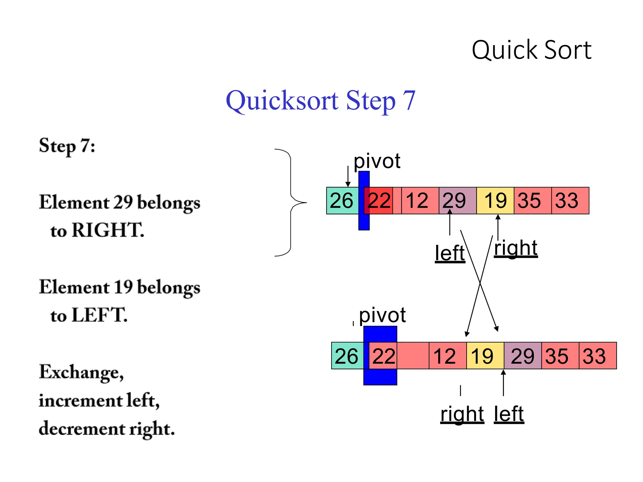
1. Pick a pivot element and partition the array into two halves based on element values relative to the pivot.
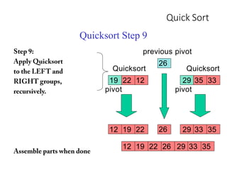
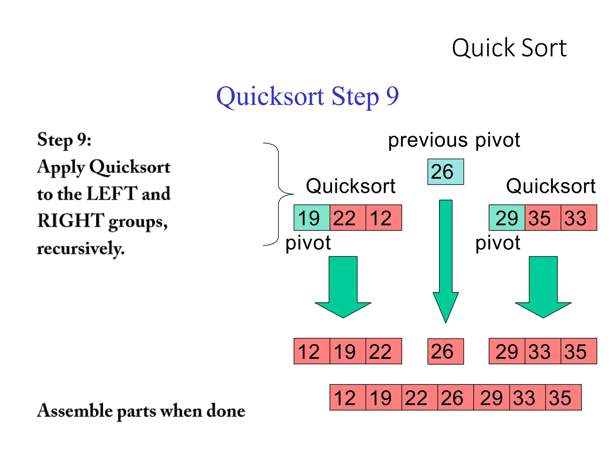
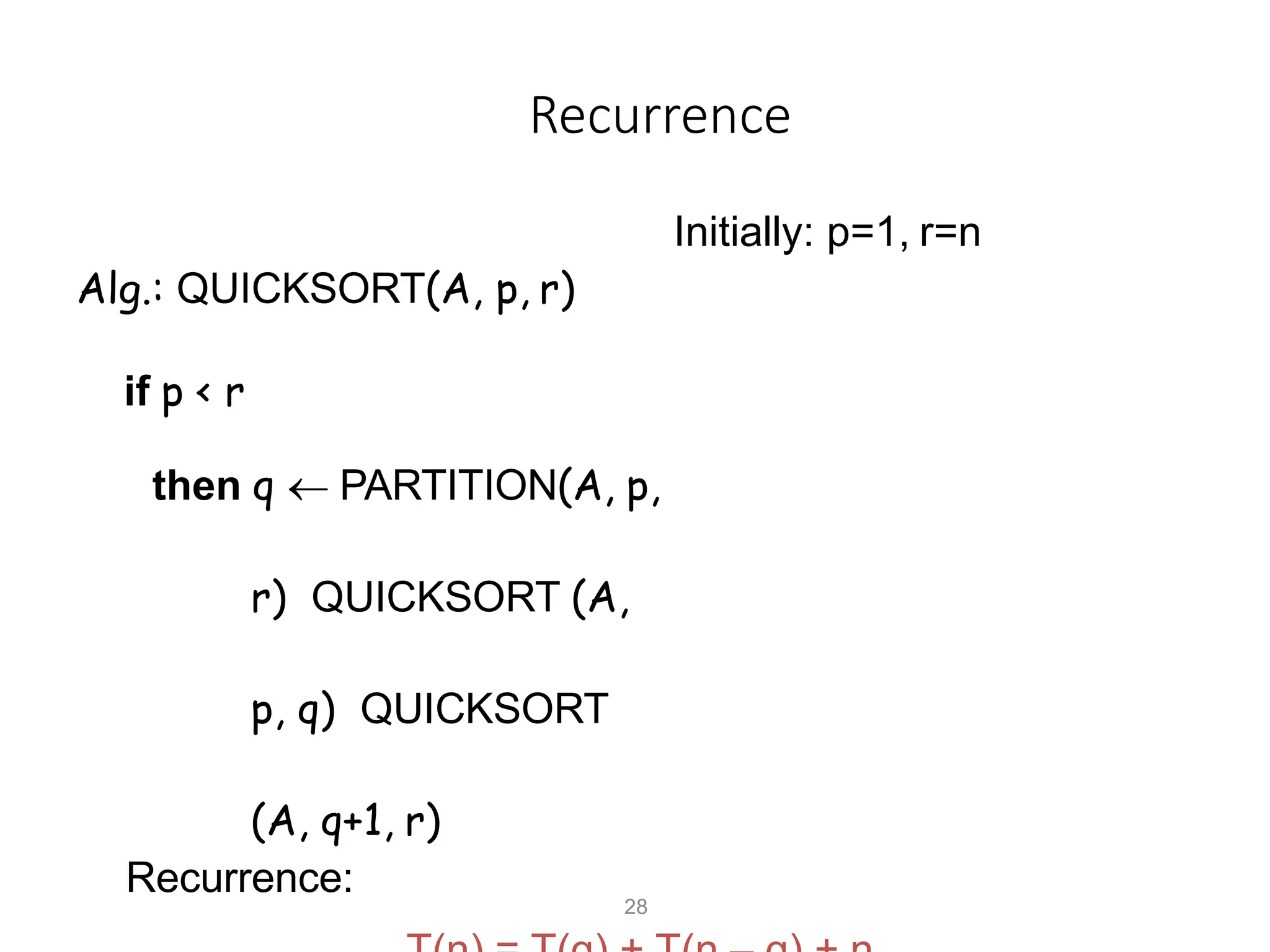
2. Recursively sort the two subarrays using quicksort.
3. The entire array is now sorted after sorting the subarrays.
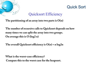
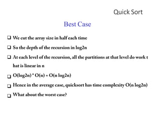
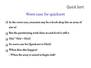
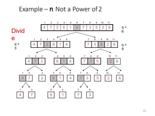
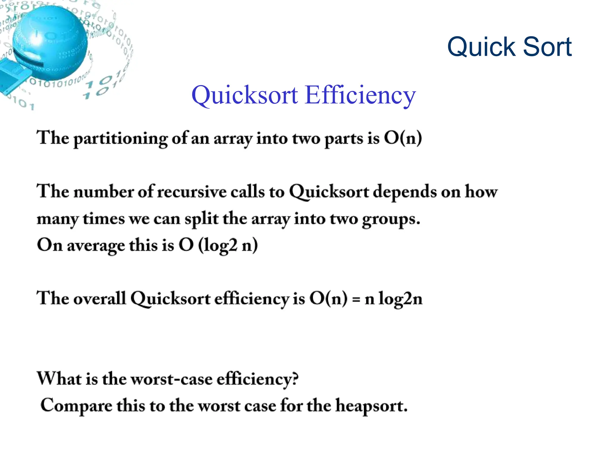
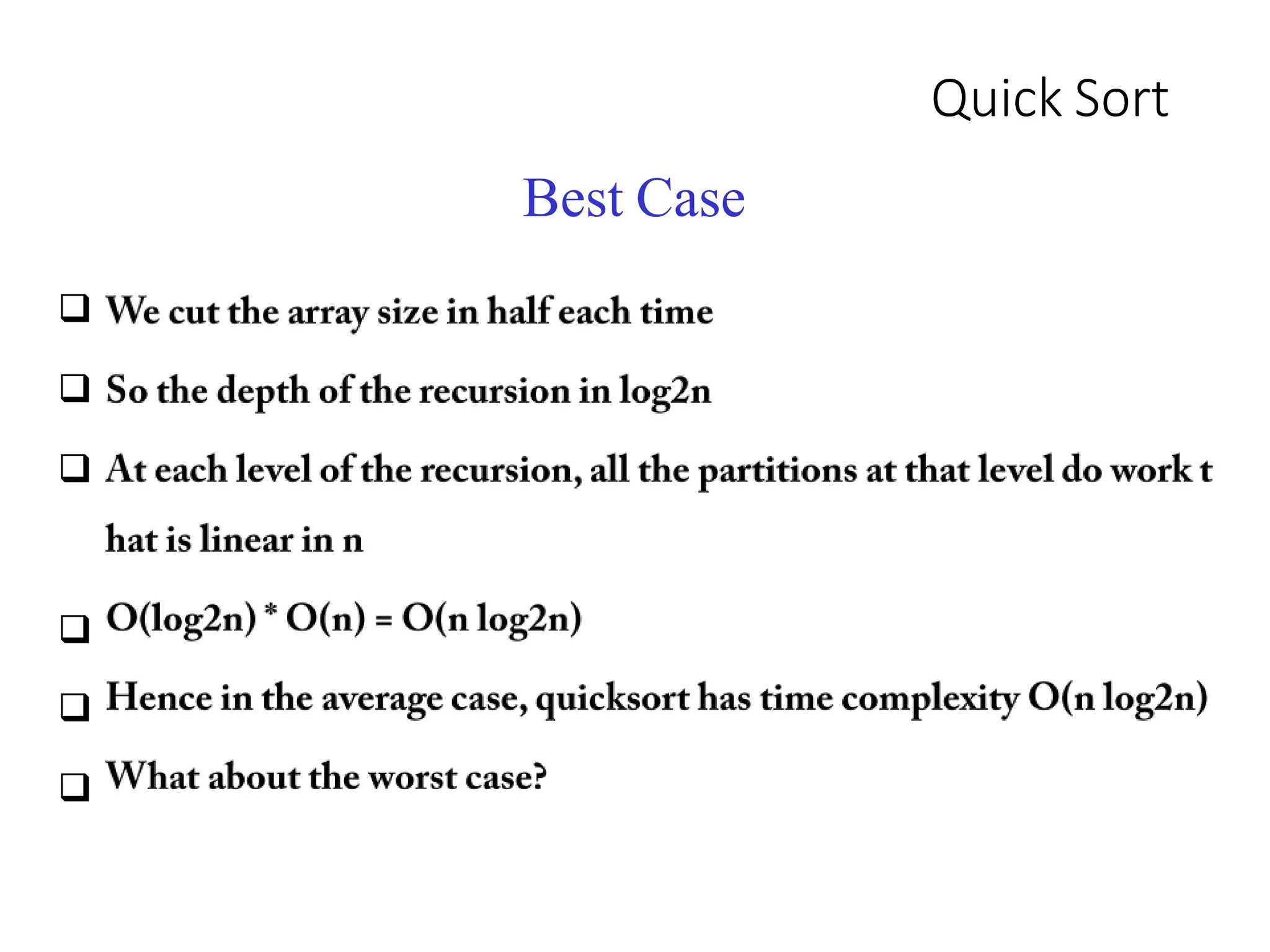
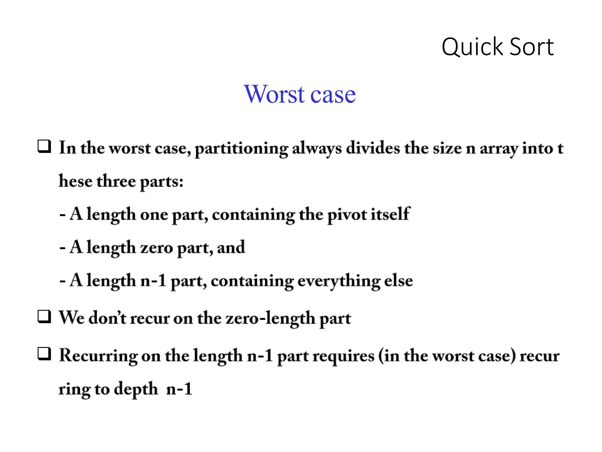
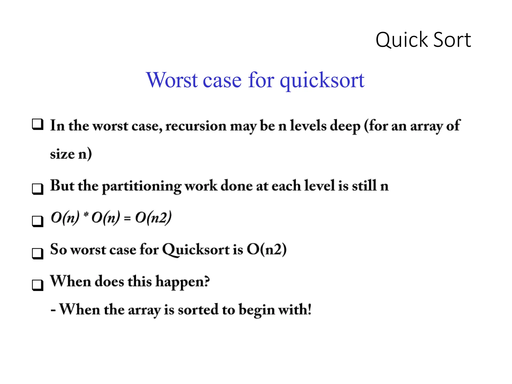
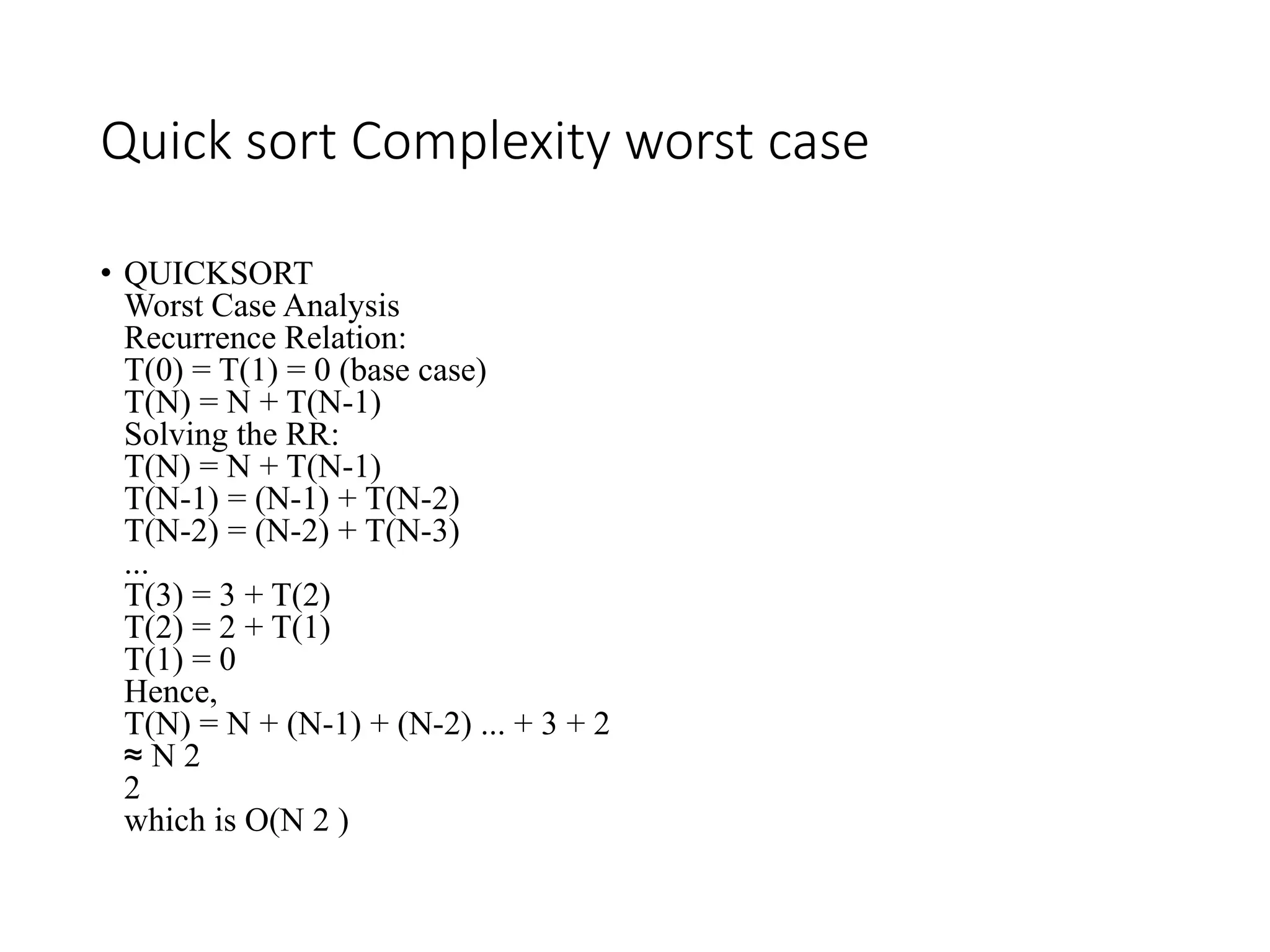
The worst case occurs when the array is already sorted or reverse sorted, taking O(n^2) time due to linear-time partitioning at each step. The average and best cases take O(nlogn) time as the array is typically partitioned close to evenly.


![1
8
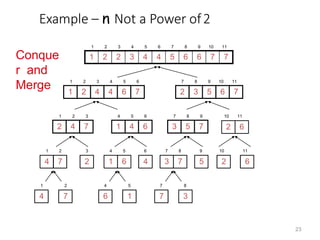
Merge Sort Approach
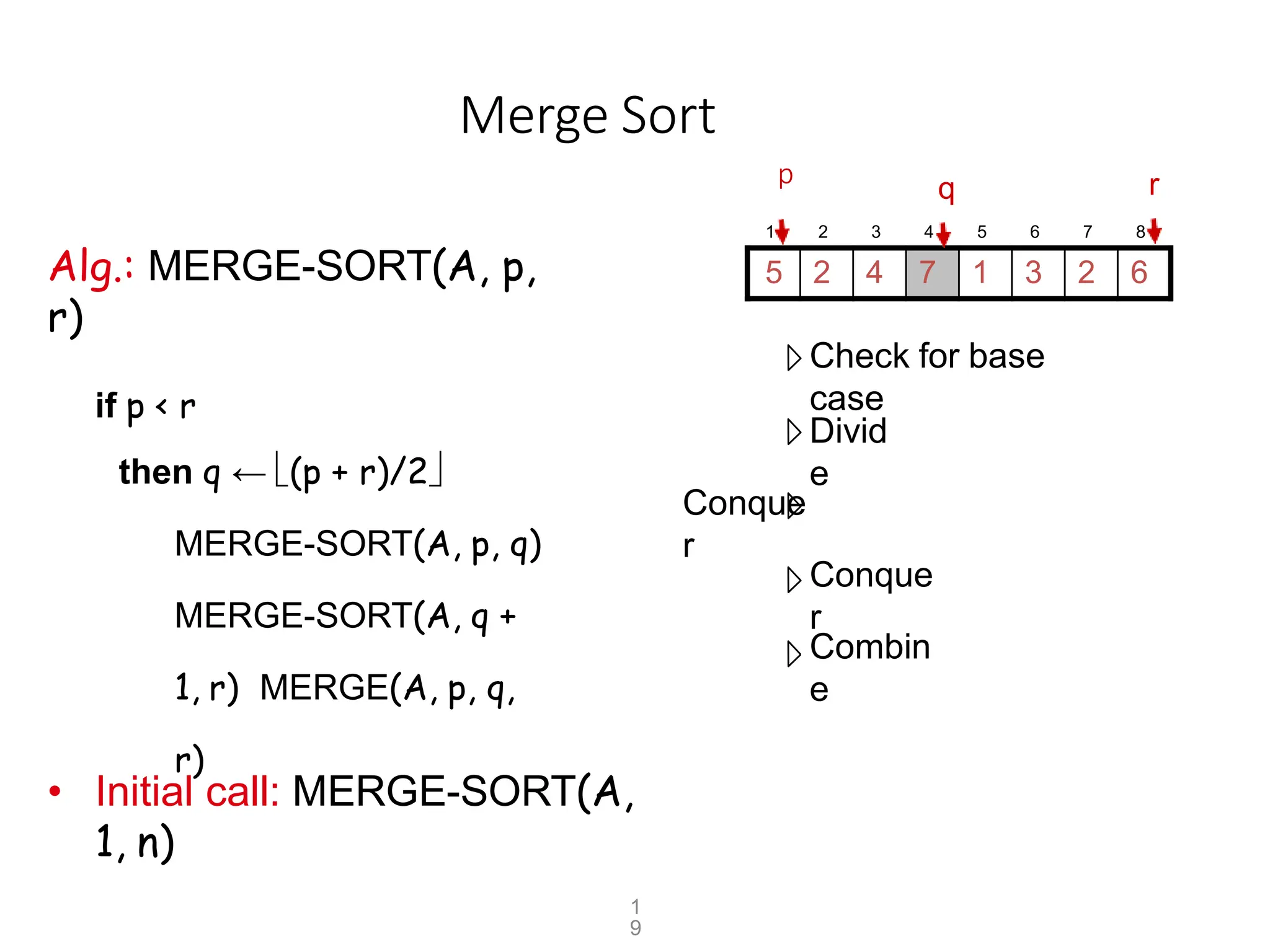
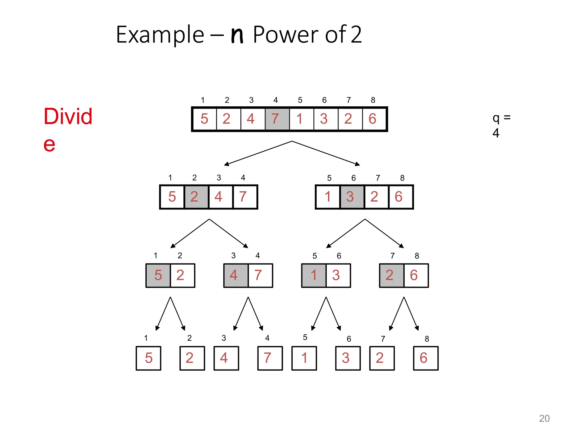
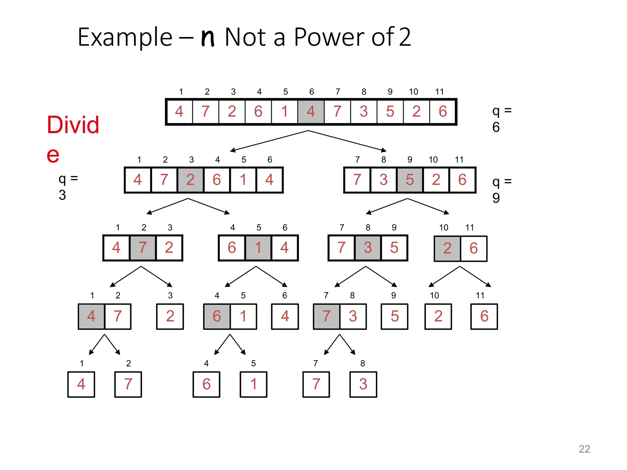
• To sort an array A[p . . r]:
• Divide
– Divide the n-element sequence to be sorted into
two subsequences of n/2 elements each
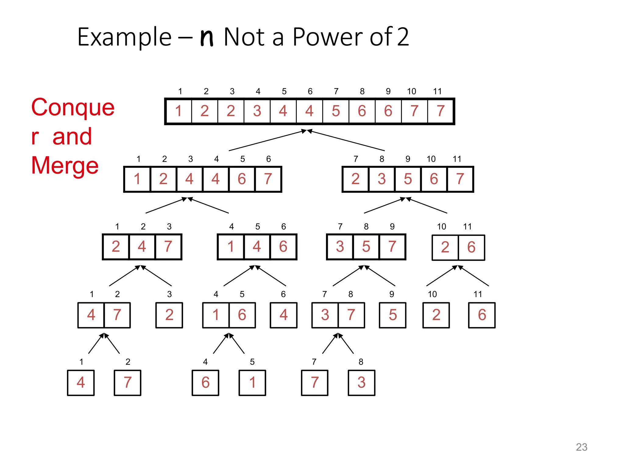
• Conquer
– Sort the subsequences recursively using merge
sort
– When the size of the sequences is 1 there is
nothing more to do
• Combine
– Merge the two sorted subsequences](https://image.slidesharecdn.com/quickandmerge-231205153646-8177edbc/85/quick-and-merge-pptx-18-320.jpg)


![11
Merge - Pseudocp
ode
Alg.: MERGE(A, p,
q, r)
1. Compute n1 and
n2
2. Copy the first n1 elements
into
. . n1 + 1] and the next n2 elements into R[1 . . n2 +
1]
3. L[n1 + 1] ← ; R[n2 + 1] ←
4. i ← 1; j ← 1
5. for k ← p to
r
6. do if L[ i ] ≤ R[ j ]
7. then A[k] ← L[ i
]
8. i ←i + 1
9. else A[k] ← R[ j
]
p q
2 4 5 7
1 2 3 6
r
q +
1
L
R
1 2 3 4 5 6 7 8
2 4 5 7 1 2 3 6
r
q
Ln2
[1
n1](https://image.slidesharecdn.com/quickandmerge-231205153646-8177edbc/85/quick-and-merge-pptx-24-320.jpg)
![Algorithm:
mergesort( int [] a, int left, int right)
{
if (right > left)
{ middle = left + (right -
left)/2; mergesort(a, left,
middle); mergesort(a,
middle+1, right); merge(a,
left, middle, right); }
}
Complexity of Merge
Sort](https://image.slidesharecdn.com/quickandmerge-231205153646-8177edbc/85/quick-and-merge-pptx-25-320.jpg)
![1
4
Quicksort
A[p…q]
• Sort an array A[p…r]
• Divide
– Partition the array A into 2 subarrays A[p..q] and A[q+1..r],
such that each element of A[p..q] is smaller than or equal to
each element in A[q+1..r]
– Need to find index q to partition the array
≤ A[q+1…r]](https://image.slidesharecdn.com/quickandmerge-231205153646-8177edbc/85/quick-and-merge-pptx-26-320.jpg)
![Quicksort
A[p…q]
• Conquer
– Recursively sort A[p..q] and A[q+1..r]using
Quicksort
• Combine
– Trivial: the arrays are sorted in place
– No additional work is required to combine them
– The entire array is now sorted
A[q+1…r]
≤
27](https://image.slidesharecdn.com/quickandmerge-231205153646-8177edbc/85/quick-and-merge-pptx-27-320.jpg)

![Partitioning the Array
Alg. PARTITION (A,
p, r)
1. x A[p]
2. i p – 1
3. j r + 1
4. while TRUE
5. do repeat j j –
1
6. until A[j] ≤ x
7. do repeat i i +
1
8. until A[i] ≥ x
9. if i < j
then exchange A[i]
A[j]
else return j
Each element
is visited
once!
Running time:
(n) n = r – p + 1
5 3 2 6 4 1 3 7
i j
A
:
ap ar
j=q i
A
:
A[p…q]
29
A[q+1…r]
≤
p r](https://image.slidesharecdn.com/quickandmerge-231205153646-8177edbc/85/quick-and-merge-pptx-29-320.jpg)


![1
8
Merge Sort Approach
• To sort an array A[p . . r]:
• Divide
– Divide the n-element sequence to be sorted into
two subsequences of n/2 elements each
• Conquer
– Sort the subsequences recursively using merge
sort
– When the size of the sequences is 1 there is
nothing more to do
• Combine
– Merge the two sorted subsequences](https://image.slidesharecdn.com/quickandmerge-231205153646-8177edbc/75/quick-and-merge-pptx-18-2048.jpg)

![11
Merge - Pseudocp
ode
Alg.: MERGE(A, p,
q, r)
1. Compute n1 and
n2
2. Copy the first n1 elements
into
. . n1 + 1] and the next n2 elements into R[1 . . n2 +
1]
3. L[n1 + 1] ← ; R[n2 + 1] ←
4. i ← 1; j ← 1
5. for k ← p to
r
6. do if L[ i ] ≤ R[ j ]
7. then A[k] ← L[ i
]
8. i ←i + 1
9. else A[k] ← R[ j
]
p q
2 4 5 7
1 2 3 6
r
q +
1
L
R
1 2 3 4 5 6 7 8
2 4 5 7 1 2 3 6
r
q
Ln2
[1
n1](https://image.slidesharecdn.com/quickandmerge-231205153646-8177edbc/75/quick-and-merge-pptx-24-2048.jpg)
![Algorithm:
mergesort( int [] a, int left, int right)
{
if (right > left)
{ middle = left + (right -
left)/2; mergesort(a, left,
middle); mergesort(a,
middle+1, right); merge(a,
left, middle, right); }
}
Complexity of Merge
Sort](https://image.slidesharecdn.com/quickandmerge-231205153646-8177edbc/75/quick-and-merge-pptx-25-2048.jpg)
![1
4
Quicksort
A[p…q]
• Sort an array A[p…r]
• Divide
– Partition the array A into 2 subarrays A[p..q] and A[q+1..r],
such that each element of A[p..q] is smaller than or equal to
each element in A[q+1..r]
– Need to find index q to partition the array
≤ A[q+1…r]](https://image.slidesharecdn.com/quickandmerge-231205153646-8177edbc/75/quick-and-merge-pptx-26-2048.jpg)
![Quicksort
A[p…q]
• Conquer
– Recursively sort A[p..q] and A[q+1..r]using
Quicksort
• Combine
– Trivial: the arrays are sorted in place
– No additional work is required to combine them
– The entire array is now sorted
A[q+1…r]
≤
27](https://image.slidesharecdn.com/quickandmerge-231205153646-8177edbc/75/quick-and-merge-pptx-27-2048.jpg)
![Partitioning the Array
Alg. PARTITION (A,
p, r)
1. x A[p]
2. i p – 1
3. j r + 1
4. while TRUE
5. do repeat j j –
1
6. until A[j] ≤ x
7. do repeat i i +
1
8. until A[i] ≥ x
9. if i < j
then exchange A[i]
A[j]
else return j
Each element
is visited
once!
Running time:
(n) n = r – p + 1
5 3 2 6 4 1 3 7
i j
A
:
ap ar
j=q i
A
:
A[p…q]
29
A[q+1…r]
≤
p r](https://image.slidesharecdn.com/quickandmerge-231205153646-8177edbc/75/quick-and-merge-pptx-29-2048.jpg)


![UNIT V Searching Sorting Hashing Techniques [Autosaved].pptx](https://cdn.slidesharecdn.com/ss_thumbnails/unitvsearchingsortinghashingtechniquesautosaved-241126054304-95a69c51-thumbnail.jpg?width=600ounds&width=560&fit=bounds)
![UNIT V Searching Sorting Hashing Techniques [Autosaved].pptx](https://cdn.slidesharecdn.com/ss_thumbnails/unitvsearchingsortinghashingtechniquesautosaved-241014040608-74caa0f6-thumbnail.jpg?width=600ounds&width=560&fit=bounds)


