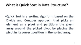
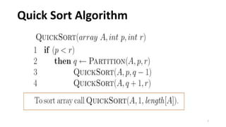
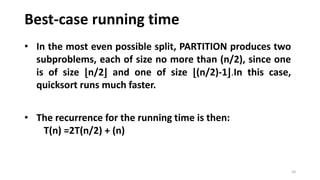
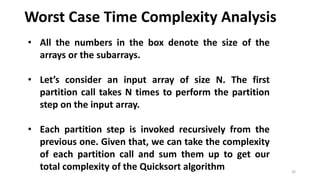
KEMBAR78
Class13_Quicksort_Algorithm.pdf
Quick Sort Algorithm
Dr J P Patra
Associate Professor
Computer Science & Engineering
UTD, CSVTU, Bhilai
1
Outline:
• What is Quick Sort in Data Structure?
• When to Use Quick Sort?
• Explanation of Quick Sort Algorithm
• Example of Quick Sort
• Time Complexity of Quick Sort
• Advantages and Disadvantages of Quick Sort
• Applications of Quick Sort
2
What is Quick Sort in Data Structure?
•Quick Sort is a sorting algorithm based on the
Divide and Conquer approach that picks an
element as a pivot and partitions the given
array around the picked pivot by placing the
pivot in its correct position in the sorted array.
3
What is Divide and Conquer approach?
4
This technique can be divided into the following 3 parts:
• Divide: This involves dividing the problem into smaller
sub-problems.
• Conquer: Solve sub-problems by calling recursively until
solved.
• Combine: Combine the sub-problems to get the final
solution of the whole problem.
5
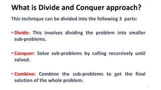
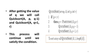
Here is the three-steps divide-and-conquer process for
sorting a typical array A[p….r].
Divide: Partition (rearrange) the array A[p.....r] into two
(possibly empty) subarrays A[p.....q - 1] and A[q+1.....r] such
that each element of A[p.....q - 1] is less than to A[q], and
each element of A[q+1......r] is greater than or equal to A[q]
Compute the index q as part of this partitioning procedure.
6
Conquer: Sort the two subarrays A[p....q - 1] and
A[q+1......r] by recursive calls to quicksort.
Combine: Since the subarrays are sorted in place, now
work is needed to combine them
So we can define that the entire array A[p....r] is now
sorted.
Quick Sort Algorithm
7
Quick Sort Partition Algorithm
8
9
• Here the value of p=1 and r=8
• As per the Partition Algorithm
the value of x=4 (As A[r]=A[8]=4)
• The value of i=0 (i.e p-1= 1-1=0)
• As per step no. 3 for loop will
start from (p=1) and it will
continue up to (r-1=8-1=7).
Example : A=[2, 8, 7, 1, 3, 5, 6, 4]
10
• A=[2, 8, 7, 1, 3, 5, 6, 4]
• Here the value of
x= 4, r=8, i=0, j=1, A[1]=2
do if (2≤ 4) Ture
• Then the value of iwill be 1 (i. e i=1)
and we have to swap :A[1] ↔ A[1]
• Output :
Process for j=1
11
• A=[2, 8, 7, 1, 3, 5, 6, 4]
• Here the value of
x= 4, r=8, i=1, j=2, A[2]=8
do if (8≤ 4) False
• Then we will skip the steps 5 and
6 and the output after
processing j=2 will be define as
• Output :
Process for j=2
12
• A=[2, 8, 7, 1, 3, 5, 6, 4]
• Here the value of
x= 4, r=8, i=1, j=3, A[3]=7
do if (7≤ 4) False
• Then we will skip the steps 5 and
6 and the output after
processing j=3 will be define as
• Output :
Process for j=3
13
• A=[2, 8, 7, 1, 3, 5, 6, 4]
• Here the value of
x= 4, r=8, i=1, j=4, A[4]=1
do if (1≤ 4) True
• Then the value of i will be 2 (i. e i=2)
and we have to swap :A[2] ↔ A[4]
• Output :
Process for j=4
14
• A=[2, 1, 7, 8, 3, 5, 6, 4]
• Here the value of
x= 4, r=8, i=2, j=5, A[5]=3
do if (3≤ 4) True
• Then the value of i will be 3 (i. e i =3)
and we have to swap :A[3] ↔ A[5]
• Output :
Process for j=5
15
• A=[2, 1, 3, 8, 7, 5, 6, 4]
• Here the value of
x= 4, r=8, i=3, j=6, A[6]=5
do if (5≤ 4) False
• Then we will skip the steps 5 and 6
and the output after processing j=6
will be define as
• Output :
Process for j=6
16
• A=[2, 1, 3, 8, 7, 5, 6, 4]
• Here the value of
x= 4, r=8, i=3, j=7, A[7]=6
do if (6 ≤ 4) False
• Then we will skip the steps 5 and 6
and the output after processing j=7
will be define as
• Output :
Process for j=7
17
• A=[2, 1, 3, 8, 7, 5, 6, 4]
or
Here the value of
x= 4, r=8, i=3, j=7, A[7]=6
Now using step 7 we have to exchange
A[i+1] ↔ A[r] i.e A[4] ↔ A[8]
Output:
Step 8 will return value 4
Process Step 7 and 8
• Using Quick Sort Partition algorithm return the value 4 and
that value will be assign to variable q.
• Now we divide the array in two sub arrays A[1…3] and
A[5….8] and the position of the Pivot element is 4.
18
Sub Array2 A[5….8]
Sub Array1 A[1….3] Position of Pivot
element
19
• After getting the value
of q we will call
Quicksort(A, p, q-1)
and Quicksort(A, q+1,
r)
• This process will
continue until we
satisfy the condition.
Best-case running time
20
• In the most even possible split, PARTITION produces two
subproblems, each of size no more than (n/2), since one
is of size ⌊n/2⌋ and one of size ⌊(n/2)-1⌋.In this case,
quicksort runs much faster.
• The recurrence for the running time is then:
T(n) =2T(n/2) + (n)
21
Here T(n) =2T(n/2) + (n)
So we can solve the above recurrence equation using
Master Method
Master Method Standard equation is T(n) =aT(n/b) + f(n)
If we compare the two equations we will obtained the
value of a=2, b=2 and f(n)=n
22
Now we have to calculate n
loga
b
=> n
log2
2
=> n
If we compare the value of f(n) and n
loga
b both values are
equal.
So, T(n) =0(f(n).logn)
=>T(n)=0(nlogn)
Best Case running time of Quick sort is 0(nlogn)
Worst-case running time
23
• The efficiency of the Quicksort algorithm very much
depends on the selection of the pivot element.
• Let’s assume the input of the Quicksort is a sorted array and
we choose the leftmost element as a pivot element.
• In this case, we’ll have two extremely unbalanced arrays.
One array will have one element and the other one will
have (N - 1) elements.
Worst-case running time
24
• Similarly, when the given input array is sorted reversely and
we choose the rightmost element as the pivot element, the
worst case occurs. Again, in this case, the pivot elements
will split the input array into two unbalanced arrays.
Worst Case Time Complexity Analysis
25
Worst Case Time Complexity Analysis
26
• All the numbers in the box denote the size of the
arrays or the subarrays.
• Let’s consider an input array of size N. The first
partition call takes N times to perform the partition
step on the input array.
• Each partition step is invoked recursively from the
previous one. Given that, we can take the complexity
of each partition call and sum them up to get our
total complexity of the Quicksort algorithm
27
Alternatively, we can create a recurrence relation for
computing it.
Or
28
• In the worst case, after the first partition, one array will
have 1 element and the other one will have (N-1)
elements.
• Let’s say T(N) denotes the time complexity to sort N
elements in the worst case:
• T(N) = Time needed to partition N elements + Time
needed to sort (N - 1) elements recursively = N + T(N - 1)
• Again for the base case when N = 0 and 1, we don’t need
to sort anything. Hence, the sorting time is 0 and T(0)=
T(1) = 0
29
Now, we’re ready to solve the recurrence relation
T(N) = N + T(N- 1),
T(N - 1) = (N - 1) + T(N- 2),
T(N - 2) = (N - 2) + T(N- 3),
T(N - 3) = (N - 3) + T(N- 4),
......
......
......
T(3) = 3 + T(2),
T(2) = 2 + T(1),
T(1) = 0
30
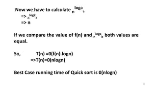
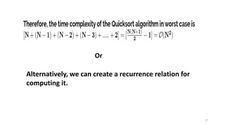
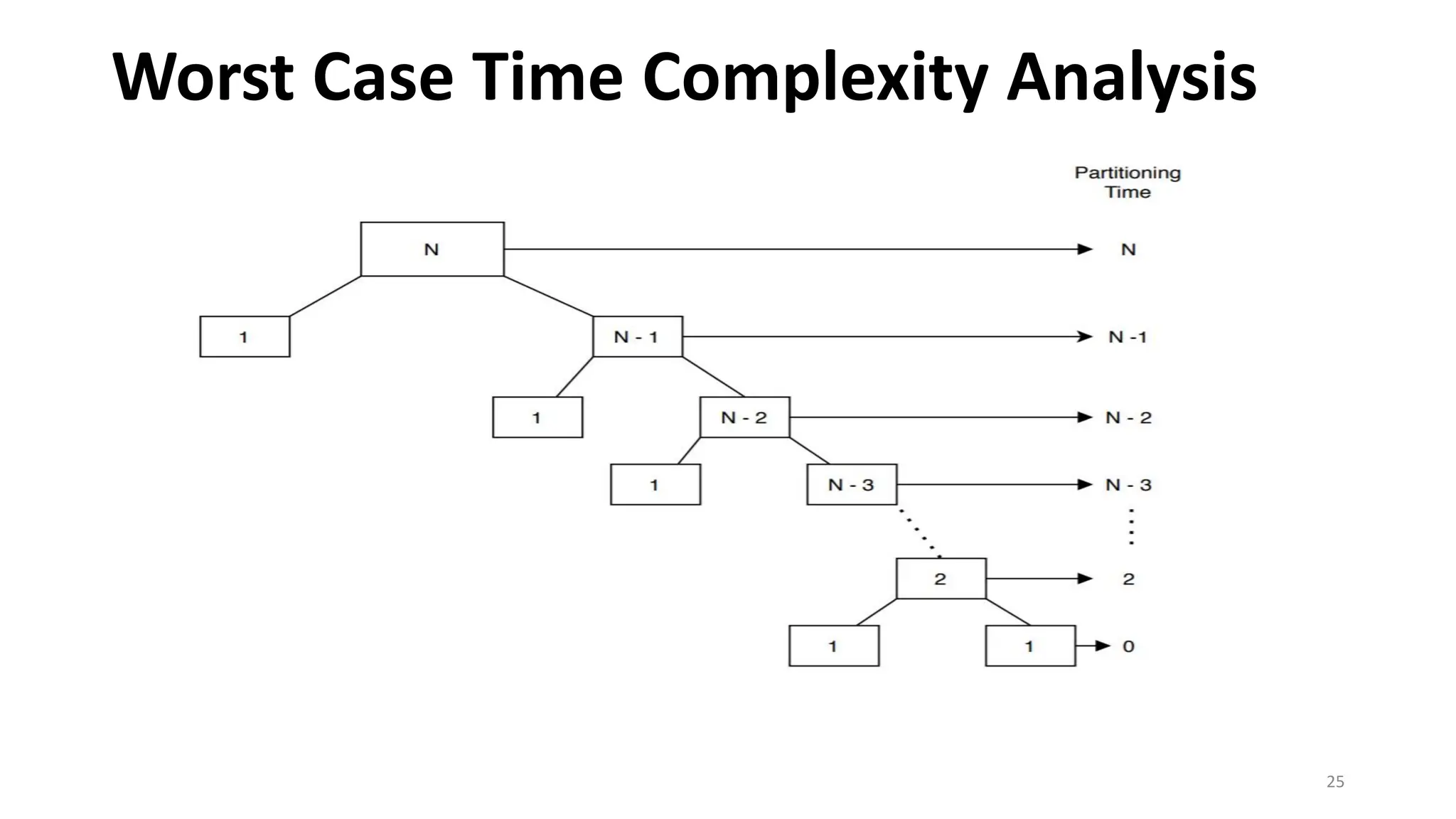
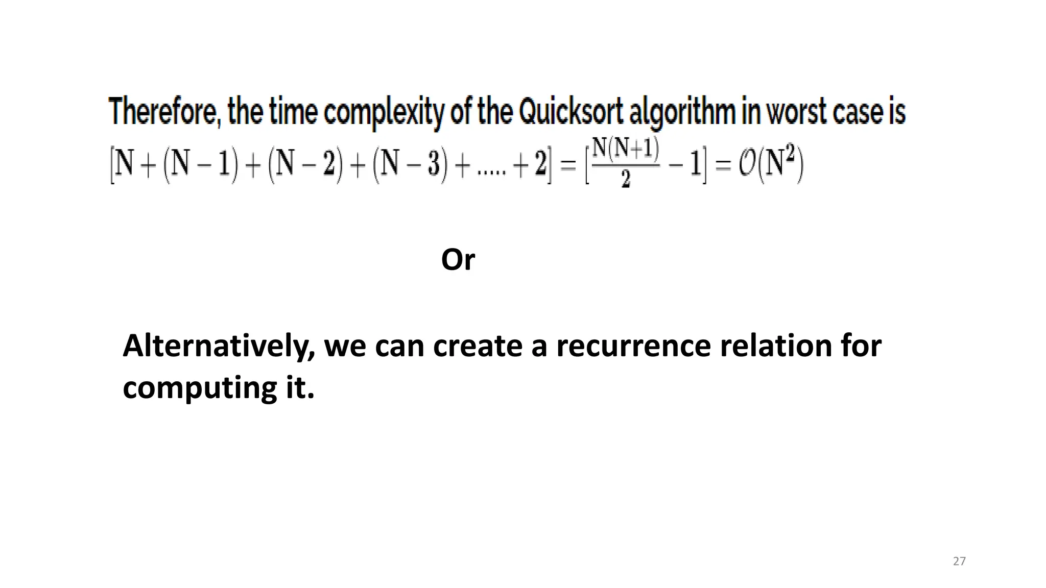
As a result, T(N) = N + (N-1) + (N-2) ... + 3 + 2
= [
𝑵(𝑵+𝟏)
𝟐
- 1] =O(N2)
Advantages of Quick Sort
31
• Fast and efficient : Quick sort is the most favored users’
choice to perform sorting functions quickly and
efficiently. It allows users to achieve the same result
much quicker than other sorting algorithms
• Cache friendly :The most talked-about feature of
quicksort is its in-place sorting. This means, at the time
of sorting, the algorithm doesn’t need additional storage
space. Thus, the sorted list occupies the same storage as
the unsorted list, and the sorting takes place in the given
area
Advantages of Quick Sort
32
• Good for parallelization: Quick sort can be parallelized
easily, taking advantage of multiple processors or
computing resources. By splitting the input array into
sub-arrays and sorting them concurrently, it can achieve
faster sorting times on systems with parallel processing
capabilities.
• Simple implementation: Quick sort's algorithmic logic is
relatively straightforward, making it easier to
understand and implement compared to some other
complex sorting algorithms
Advantages of Quick Sort
33
• Time complexity: Time complexity is the time taken by
the algorithm to run until its completion. Compared to
other sorting algorithms, it can be said that the time
complexity of quick sort is the best
• Space complexity: Quick sort has a space complexity of
O(logn), making it a suitable algorithm when you have
restrictions in space availability
Disadvantages of Quick Sort
34
• Unstable: Quick sort is undoubtedly a fast and efficient
sorting algorithm, but when it comes to stability, you
might want to reconsider your options. This sorting
algorithm is regarded unstable as it does not retain the
original order of the key-value pair.
• Worst-case time complexity: This is actually a drawback
of quick sort. It usually occurs when the element
selected as the pivot is the largest or smallest element,
or when all the elements are the same. These worst
cases drastically affect the performance of the quick
sort.
Disadvantages of Quick Sort
35
• Dependency on Pivot Selection: The choice of pivot
significantly affects the performance of quick sort. If a poorly
chosen pivot divides the array into highly imbalanced
partitions, the algorithm's efficiency may degrade. This issue
is particularly prominent when dealing with already sorted or
nearly sorted arrays.
• Recursive Overhead: Quick sort heavily relies on recursion to
divide the array into subarrays. Recursive function calls
consume additional memory and can lead to stack overflow
errors when dealing with large data sets. This makes quick
sort less suitable for sorting extremely large arrays.
Disadvantages of Quick Sort
36
• Inefficient for Small Data Sets: Quick sort has additional
overhead in comparison to some simpler sorting algorithms,
especially when dealing with small data sets. The recursive
nature of quick sort and the constant splitting of the array can
be inefficient for sorting small arrays or arrays with a small
number of unique elements.
• Not Adaptive: Quick sort's performance is not adaptive to the
initial order of the elements. It does not take advantage of any
pre-existing order or partially sorted input. This means that
even if a portion of the array is already sorted, the quick sort
will still perform partitioning operations on the entire array.
Applications of Quick Sort
37
• Commercial Computing is used in various government and
private organizations for the purpose of sorting various
data like sorting files by name/date/price, sorting of
students by their roll no., sorting of account profile by given
id, etc.
• The sorting algorithm is used for information searching and
as Quicksort is the fastest algorithm so it is widely used as a
better way of searching.
• It is used everywhere where a stable sort is not needed.
Applications of Quick Sort
38
• Quicksort is a cache-friendly algorithm as it has a good
locality of reference when used for arrays.
• It is tail -recursive and hence all the call optimization can be
done.
• It is used to implement primitive type methods.
• It is used in operational research and event-driven
simulation.
39
Conclusion:
Overall, quick sort is a powerful data structure algorithm
with advantages such as efficiency and versatility. It is an
essential tool for developers to have in their belt when
dealing with large amounts of data. Quicksort is an
efficient, unstable sorting algorithm with time
complexity of O(n log n) in the best and average case
and O(n²) in the worst case.
40

Class13_Quicksort_Algorithm.pdf

  • 1.
    Quick Sort Algorithm DrJ P Patra Associate Professor Computer Science & Engineering UTD, CSVTU, Bhilai 1
  • 2.
    Outline: • What isQuick Sort in Data Structure? • When to Use Quick Sort? • Explanation of Quick Sort Algorithm • Example of Quick Sort • Time Complexity of Quick Sort • Advantages and Disadvantages of Quick Sort • Applications of Quick Sort 2
  • 3.
    What is QuickSort in Data Structure? •Quick Sort is a sorting algorithm based on the Divide and Conquer approach that picks an element as a pivot and partitions the given array around the picked pivot by placing the pivot in its correct position in the sorted array. 3
  • 4.
    What is Divideand Conquer approach? 4 This technique can be divided into the following 3 parts: • Divide: This involves dividing the problem into smaller sub-problems. • Conquer: Solve sub-problems by calling recursively until solved. • Combine: Combine the sub-problems to get the final solution of the whole problem.
  • 5.
    5 Here is thethree-steps divide-and-conquer process for sorting a typical array A[p….r]. Divide: Partition (rearrange) the array A[p.....r] into two (possibly empty) subarrays A[p.....q - 1] and A[q+1.....r] such that each element of A[p.....q - 1] is less than to A[q], and each element of A[q+1......r] is greater than or equal to A[q] Compute the index q as part of this partitioning procedure.
  • 6.
    6 Conquer: Sort thetwo subarrays A[p....q - 1] and A[q+1......r] by recursive calls to quicksort. Combine: Since the subarrays are sorted in place, now work is needed to combine them So we can define that the entire array A[p....r] is now sorted.
  • 7.
  • 8.
  • 9.
    9 • Here thevalue of p=1 and r=8 • As per the Partition Algorithm the value of x=4 (As A[r]=A[8]=4) • The value of i=0 (i.e p-1= 1-1=0) • As per step no. 3 for loop will start from (p=1) and it will continue up to (r-1=8-1=7). Example : A=[2, 8, 7, 1, 3, 5, 6, 4]
  • 10.
    10 • A=[2, 8,7, 1, 3, 5, 6, 4] • Here the value of x= 4, r=8, i=0, j=1, A[1]=2 do if (2≤ 4) Ture • Then the value of iwill be 1 (i. e i=1) and we have to swap :A[1] ↔ A[1] • Output : Process for j=1
  • 11.
    11 • A=[2, 8,7, 1, 3, 5, 6, 4] • Here the value of x= 4, r=8, i=1, j=2, A[2]=8 do if (8≤ 4) False • Then we will skip the steps 5 and 6 and the output after processing j=2 will be define as • Output : Process for j=2
  • 12.
    12 • A=[2, 8,7, 1, 3, 5, 6, 4] • Here the value of x= 4, r=8, i=1, j=3, A[3]=7 do if (7≤ 4) False • Then we will skip the steps 5 and 6 and the output after processing j=3 will be define as • Output : Process for j=3
  • 13.
    13 • A=[2, 8,7, 1, 3, 5, 6, 4] • Here the value of x= 4, r=8, i=1, j=4, A[4]=1 do if (1≤ 4) True • Then the value of i will be 2 (i. e i=2) and we have to swap :A[2] ↔ A[4] • Output : Process for j=4
  • 14.
    14 • A=[2, 1,7, 8, 3, 5, 6, 4] • Here the value of x= 4, r=8, i=2, j=5, A[5]=3 do if (3≤ 4) True • Then the value of i will be 3 (i. e i =3) and we have to swap :A[3] ↔ A[5] • Output : Process for j=5
  • 15.
    15 • A=[2, 1,3, 8, 7, 5, 6, 4] • Here the value of x= 4, r=8, i=3, j=6, A[6]=5 do if (5≤ 4) False • Then we will skip the steps 5 and 6 and the output after processing j=6 will be define as • Output : Process for j=6
  • 16.
    16 • A=[2, 1,3, 8, 7, 5, 6, 4] • Here the value of x= 4, r=8, i=3, j=7, A[7]=6 do if (6 ≤ 4) False • Then we will skip the steps 5 and 6 and the output after processing j=7 will be define as • Output : Process for j=7
  • 17.
    17 • A=[2, 1,3, 8, 7, 5, 6, 4] or Here the value of x= 4, r=8, i=3, j=7, A[7]=6 Now using step 7 we have to exchange A[i+1] ↔ A[r] i.e A[4] ↔ A[8] Output: Step 8 will return value 4 Process Step 7 and 8
  • 18.
    • Using QuickSort Partition algorithm return the value 4 and that value will be assign to variable q. • Now we divide the array in two sub arrays A[1…3] and A[5….8] and the position of the Pivot element is 4. 18 Sub Array2 A[5….8] Sub Array1 A[1….3] Position of Pivot element
  • 19.
    19 • After gettingthe value of q we will call Quicksort(A, p, q-1) and Quicksort(A, q+1, r) • This process will continue until we satisfy the condition.
  • 20.
    Best-case running time 20 •In the most even possible split, PARTITION produces two subproblems, each of size no more than (n/2), since one is of size ⌊n/2⌋ and one of size ⌊(n/2)-1⌋.In this case, quicksort runs much faster. • The recurrence for the running time is then: T(n) =2T(n/2) + (n)
  • 21.
    21 Here T(n) =2T(n/2)+ (n) So we can solve the above recurrence equation using Master Method Master Method Standard equation is T(n) =aT(n/b) + f(n) If we compare the two equations we will obtained the value of a=2, b=2 and f(n)=n
  • 22.
    22 Now we haveto calculate n loga b => n log2 2 => n If we compare the value of f(n) and n loga b both values are equal. So, T(n) =0(f(n).logn) =>T(n)=0(nlogn) Best Case running time of Quick sort is 0(nlogn)
  • 23.
    Worst-case running time 23 •The efficiency of the Quicksort algorithm very much depends on the selection of the pivot element. • Let’s assume the input of the Quicksort is a sorted array and we choose the leftmost element as a pivot element. • In this case, we’ll have two extremely unbalanced arrays. One array will have one element and the other one will have (N - 1) elements.
  • 24.
    Worst-case running time 24 •Similarly, when the given input array is sorted reversely and we choose the rightmost element as the pivot element, the worst case occurs. Again, in this case, the pivot elements will split the input array into two unbalanced arrays.
  • 25.
    Worst Case TimeComplexity Analysis 25
  • 26.
    Worst Case TimeComplexity Analysis 26 • All the numbers in the box denote the size of the arrays or the subarrays. • Let’s consider an input array of size N. The first partition call takes N times to perform the partition step on the input array. • Each partition step is invoked recursively from the previous one. Given that, we can take the complexity of each partition call and sum them up to get our total complexity of the Quicksort algorithm
  • 27.
    27 Alternatively, we cancreate a recurrence relation for computing it. Or
  • 28.
    28 • In theworst case, after the first partition, one array will have 1 element and the other one will have (N-1) elements. • Let’s say T(N) denotes the time complexity to sort N elements in the worst case: • T(N) = Time needed to partition N elements + Time needed to sort (N - 1) elements recursively = N + T(N - 1) • Again for the base case when N = 0 and 1, we don’t need to sort anything. Hence, the sorting time is 0 and T(0)= T(1) = 0
  • 29.
    29 Now, we’re readyto solve the recurrence relation T(N) = N + T(N- 1), T(N - 1) = (N - 1) + T(N- 2), T(N - 2) = (N - 2) + T(N- 3), T(N - 3) = (N - 3) + T(N- 4), ...... ...... ...... T(3) = 3 + T(2), T(2) = 2 + T(1), T(1) = 0
  • 30.
    30 As a result,T(N) = N + (N-1) + (N-2) ... + 3 + 2 = [ 𝑵(𝑵+𝟏) 𝟐 - 1] =O(N2)
  • 31.
    Advantages of QuickSort 31 • Fast and efficient : Quick sort is the most favored users’ choice to perform sorting functions quickly and efficiently. It allows users to achieve the same result much quicker than other sorting algorithms • Cache friendly :The most talked-about feature of quicksort is its in-place sorting. This means, at the time of sorting, the algorithm doesn’t need additional storage space. Thus, the sorted list occupies the same storage as the unsorted list, and the sorting takes place in the given area
  • 32.
    Advantages of QuickSort 32 • Good for parallelization: Quick sort can be parallelized easily, taking advantage of multiple processors or computing resources. By splitting the input array into sub-arrays and sorting them concurrently, it can achieve faster sorting times on systems with parallel processing capabilities. • Simple implementation: Quick sort's algorithmic logic is relatively straightforward, making it easier to understand and implement compared to some other complex sorting algorithms
  • 33.
    Advantages of QuickSort 33 • Time complexity: Time complexity is the time taken by the algorithm to run until its completion. Compared to other sorting algorithms, it can be said that the time complexity of quick sort is the best • Space complexity: Quick sort has a space complexity of O(logn), making it a suitable algorithm when you have restrictions in space availability
  • 34.
    Disadvantages of QuickSort 34 • Unstable: Quick sort is undoubtedly a fast and efficient sorting algorithm, but when it comes to stability, you might want to reconsider your options. This sorting algorithm is regarded unstable as it does not retain the original order of the key-value pair. • Worst-case time complexity: This is actually a drawback of quick sort. It usually occurs when the element selected as the pivot is the largest or smallest element, or when all the elements are the same. These worst cases drastically affect the performance of the quick sort.
  • 35.
    Disadvantages of QuickSort 35 • Dependency on Pivot Selection: The choice of pivot significantly affects the performance of quick sort. If a poorly chosen pivot divides the array into highly imbalanced partitions, the algorithm's efficiency may degrade. This issue is particularly prominent when dealing with already sorted or nearly sorted arrays. • Recursive Overhead: Quick sort heavily relies on recursion to divide the array into subarrays. Recursive function calls consume additional memory and can lead to stack overflow errors when dealing with large data sets. This makes quick sort less suitable for sorting extremely large arrays.
  • 36.
    Disadvantages of QuickSort 36 • Inefficient for Small Data Sets: Quick sort has additional overhead in comparison to some simpler sorting algorithms, especially when dealing with small data sets. The recursive nature of quick sort and the constant splitting of the array can be inefficient for sorting small arrays or arrays with a small number of unique elements. • Not Adaptive: Quick sort's performance is not adaptive to the initial order of the elements. It does not take advantage of any pre-existing order or partially sorted input. This means that even if a portion of the array is already sorted, the quick sort will still perform partitioning operations on the entire array.
  • 37.
    Applications of QuickSort 37 • Commercial Computing is used in various government and private organizations for the purpose of sorting various data like sorting files by name/date/price, sorting of students by their roll no., sorting of account profile by given id, etc. • The sorting algorithm is used for information searching and as Quicksort is the fastest algorithm so it is widely used as a better way of searching. • It is used everywhere where a stable sort is not needed.
  • 38.
    Applications of QuickSort 38 • Quicksort is a cache-friendly algorithm as it has a good locality of reference when used for arrays. • It is tail -recursive and hence all the call optimization can be done. • It is used to implement primitive type methods. • It is used in operational research and event-driven simulation.
  • 39.
    39 Conclusion: Overall, quick sortis a powerful data structure algorithm with advantages such as efficiency and versatility. It is an essential tool for developers to have in their belt when dealing with large amounts of data. Quicksort is an efficient, unstable sorting algorithm with time complexity of O(n log n) in the best and average case and O(n²) in the worst case.
  • 40.