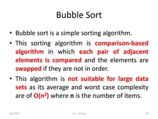
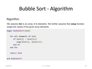
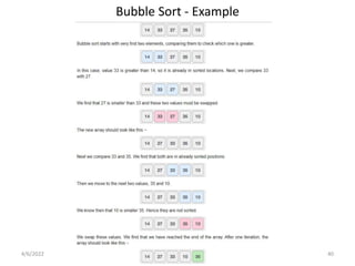
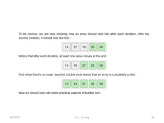
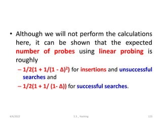
Downloaded 19 times


![Insertion Sort - Algorithm
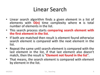
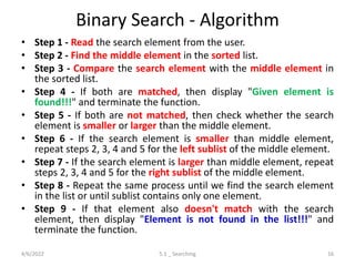
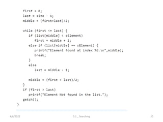
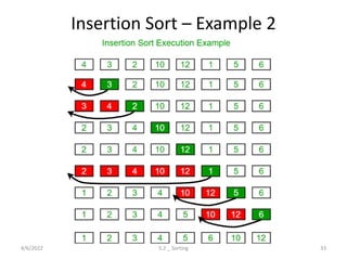
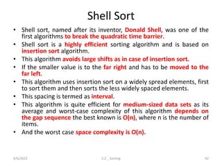
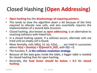
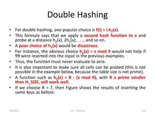
• To sort an array of size n in ascending order:
– 1: Iterate from arr[1] to arr[n] over the array.
– 2: Compare the current element (key) to its
predecessor.
– 3: If the key element is smaller than its
predecessor, compare it to the elements before.
Move the greater elements one position up to
make space for the swapped element.
4/6/2022 5.2 _ Sorting 30](https://image.slidesharecdn.com/unit5complete-211228094735/85/Searching-Sorting-and-Hashing-Techniques-30-320.jpg)

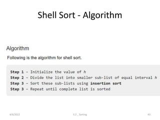
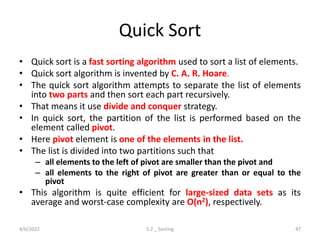
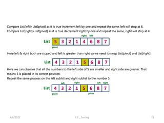
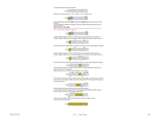
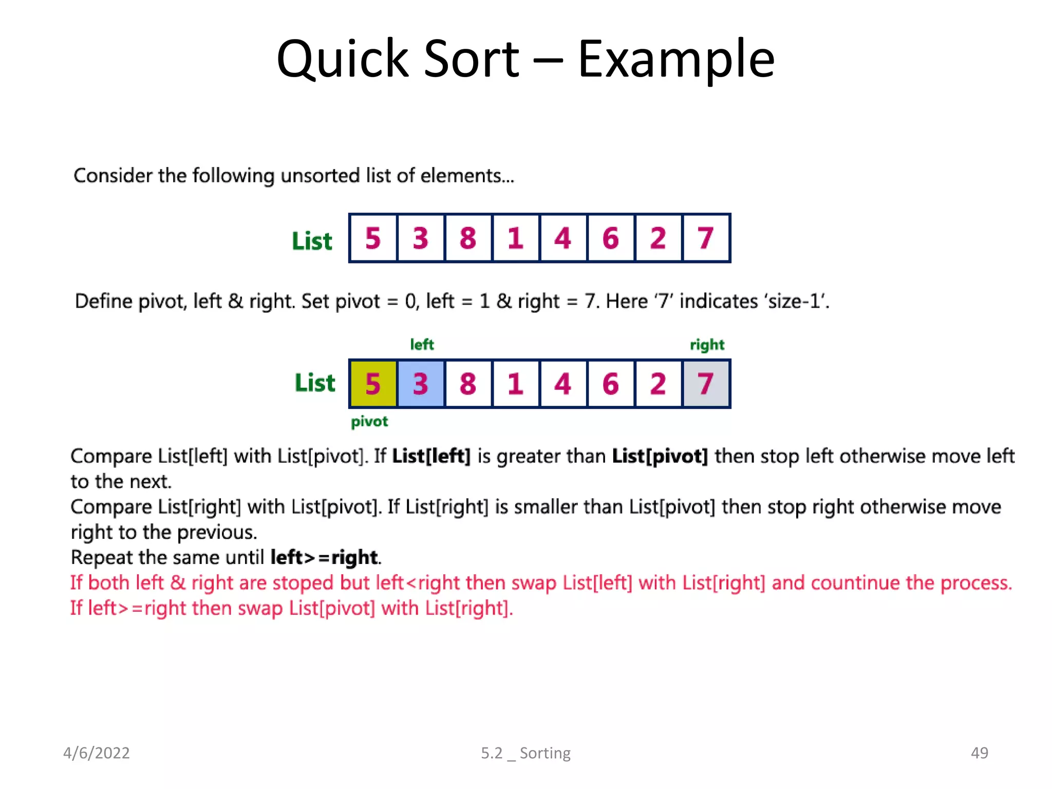
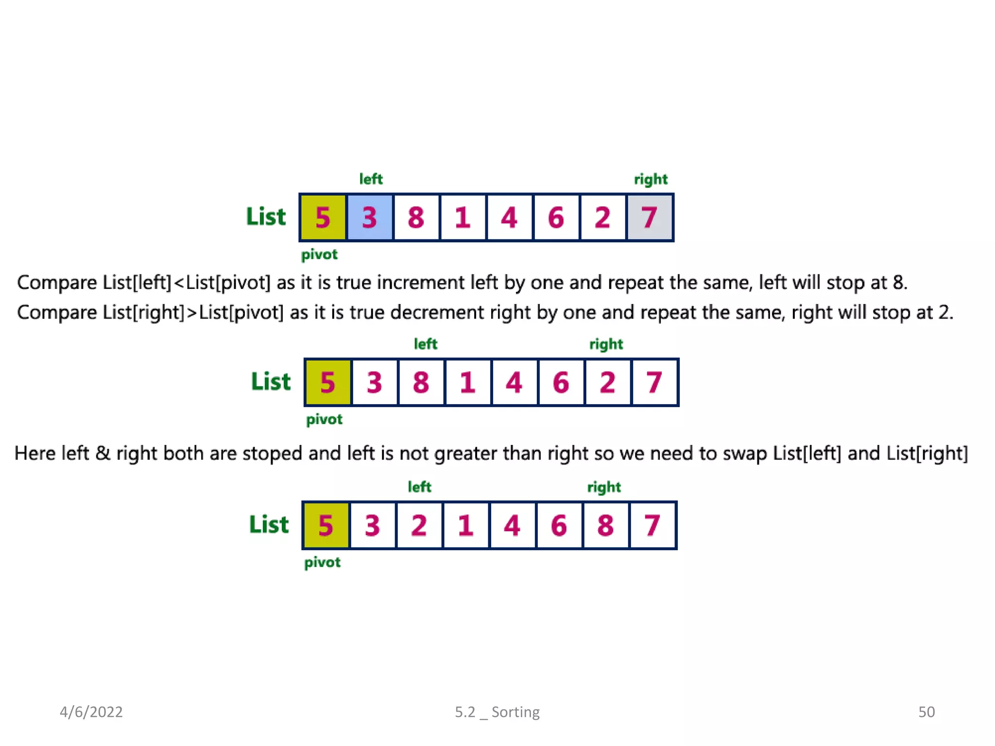
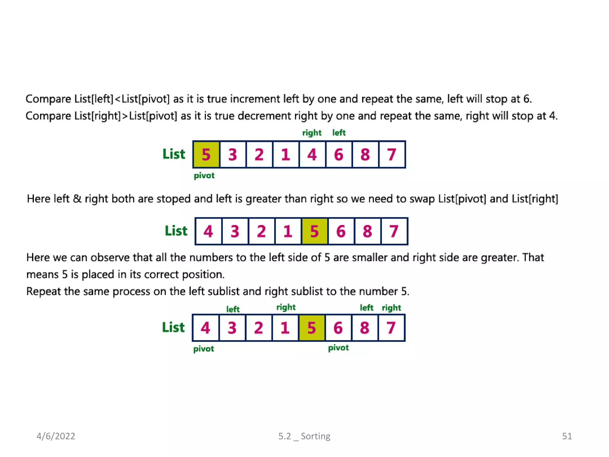
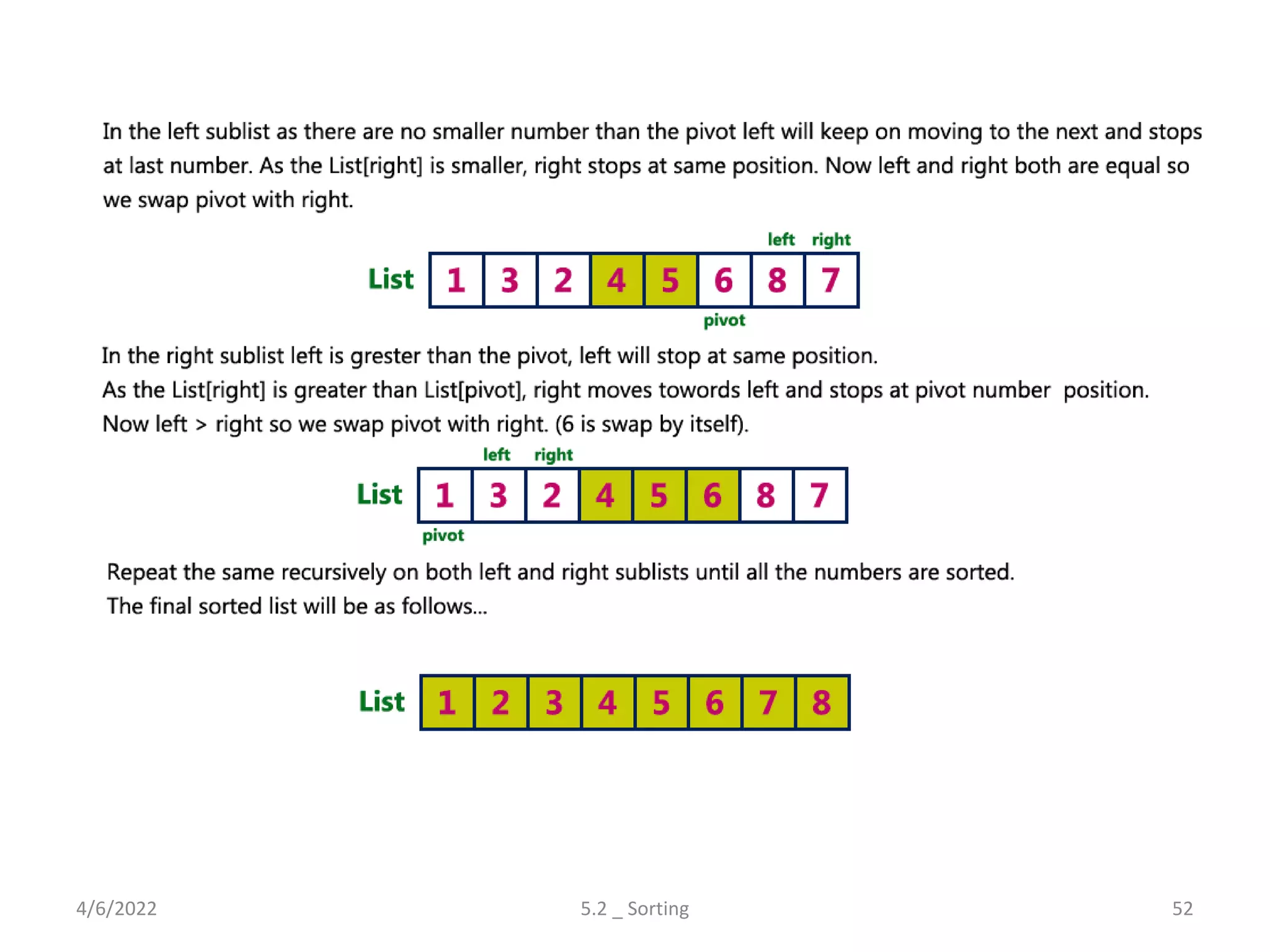
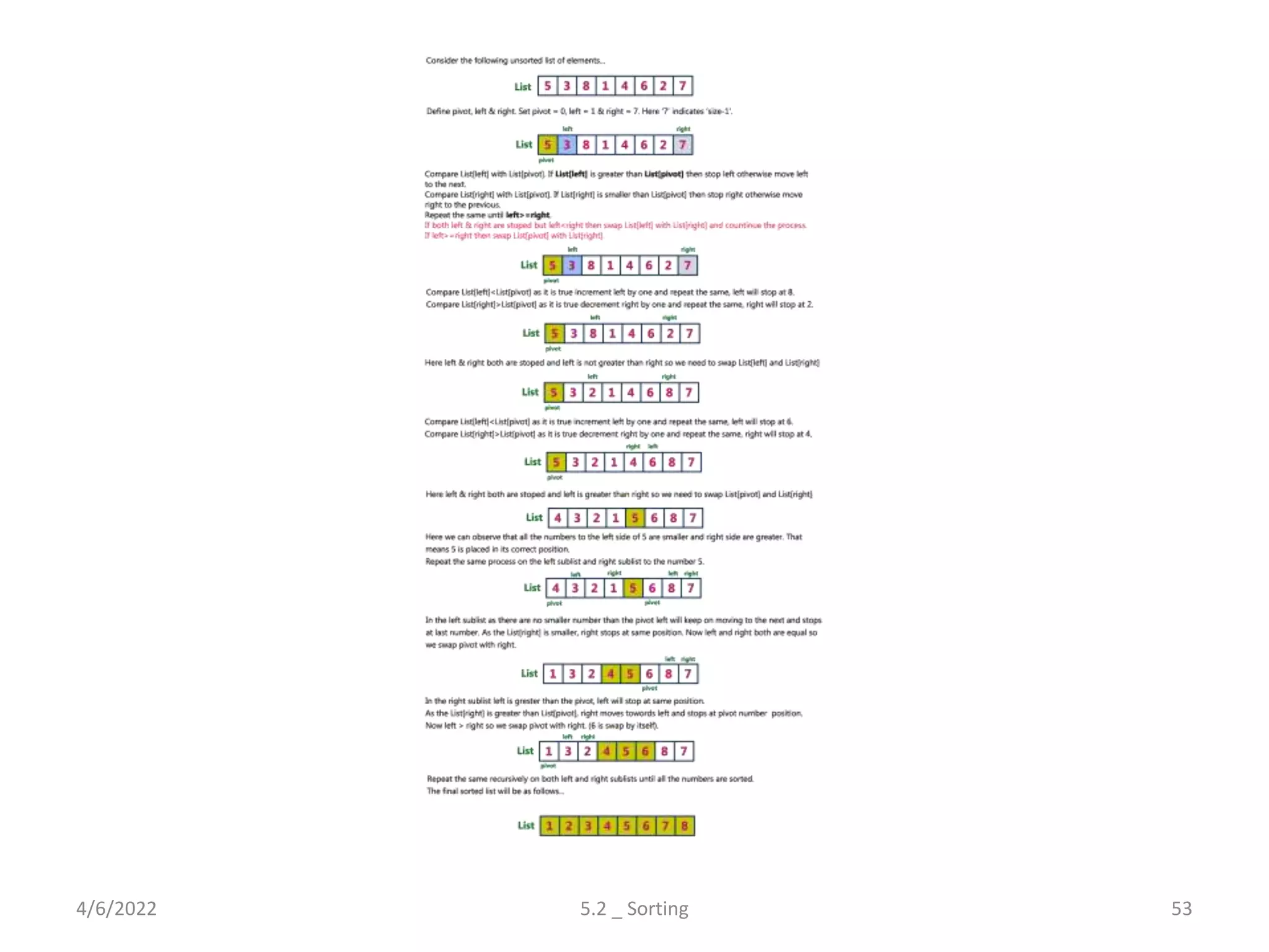
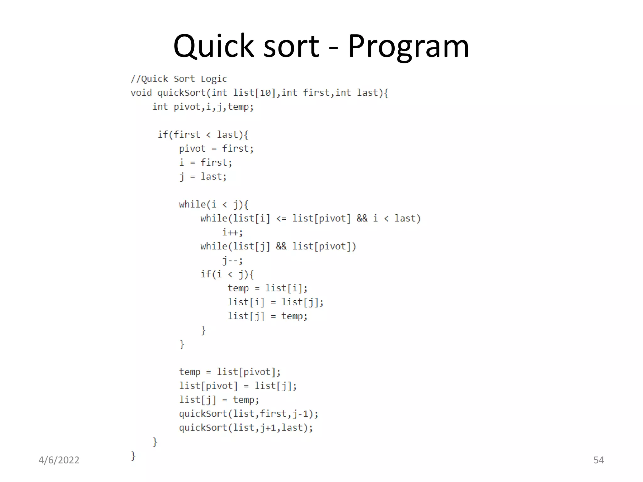
![Quick Sort – Algorithm(Pivot)
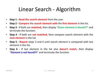
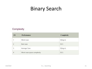
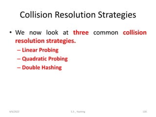
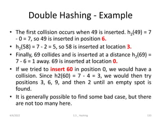
• Step 1 - Consider the first element of the list as pivot (i.e., Element at first
position in the list).
• Step 2 - Define two variables i and j. Set i and j to first and last elements of
the list respectively.
• Step 3 - Increment i until list[i] > pivot then stop.
• Step 4 - Decrement j until list[j] < pivot then stop.
• Step 5 - If i < j then exchange list[i] and list[j].
• Step 6 - Repeat steps 3,4 & 5 until i > j.
• Step 7 - Exchange the pivot element with list[j] element.
4/6/2022 5.2 _ Sorting 48](https://image.slidesharecdn.com/unit5complete-211228094735/85/Searching-Sorting-and-Hashing-Techniques-48-320.jpg)


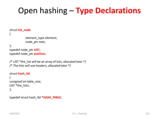
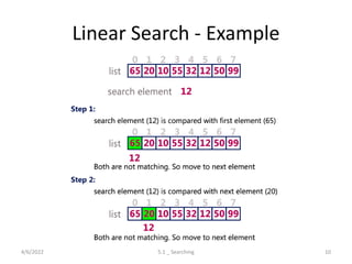
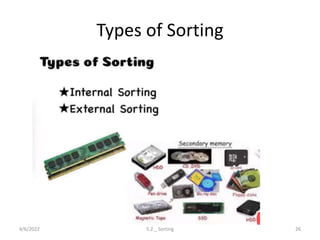
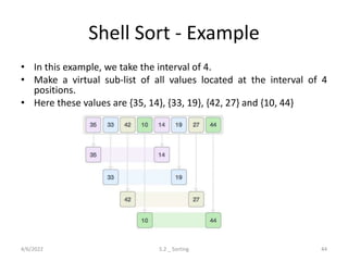
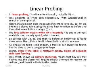
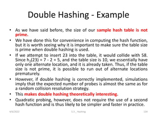
![Open hashing – Initialization
• HASH_TABLE initialize_table( unsigned int table_size )
• {
• HASH_TABLE H;
• int i;
• /*1*/ if( table size < MIN_TABLE_SIZE )
• {
• /*2*/ error("Table size too small");
• /*3*/ return NULL;
• }
• /* Allocate table */
• /*4*/ H = (HASH_TABLE) malloc ( sizeof (struct hash_tbl) );
• /*5*/ if( H == NULL )
• /*6*/ fatal_error("Out of space!!!");
• /*7*/ H->table_size = next_prime( table_size );
• /* Allocate list pointers */
• /*8*/ H->the_lists = (position *) malloc( sizeof (LIST) * H->table_size );
• /*9*/ if( H->the_lists == NULL )
• /*10*/ fatal_error("Out of space!!!");
• /* Allocate list headers */
• /*11*/ for(i=0; i<H->table_size; i++ )
• {
• /*12*/ H->the_lists[i] = (LIST) malloc( sizeof (struct list_node) );
• /*13*/ if( H->the_lists[i] == NULL )
• /*14*/ fatal_error("Out of space!!!");
• else
• /*15*/ H->the_lists[i]->next = NULL;
• }
• /*16*/ return H;
• }
4/6/2022 5.3 _ Hashing 113](https://image.slidesharecdn.com/unit5complete-211228094735/85/Searching-Sorting-and-Hashing-Techniques-113-320.jpg)
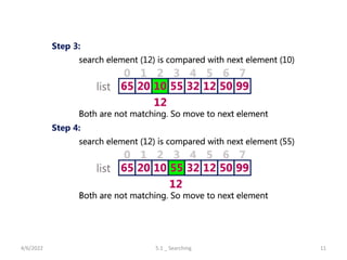
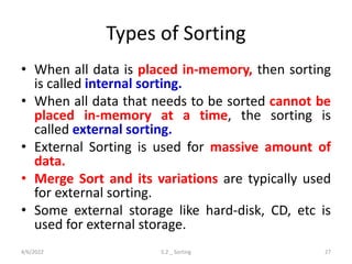
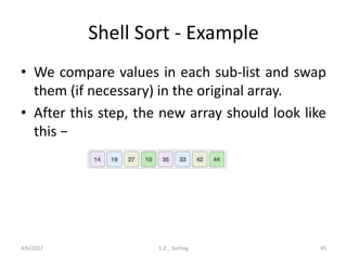
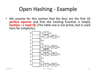
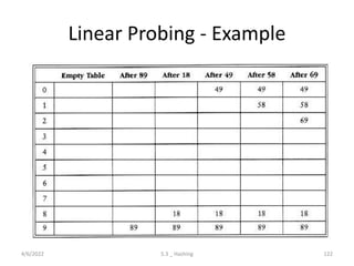
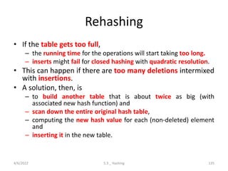
![Open Hashing – Find Routine
• position find( element_type key, HASH_TABLE H )
• {
• position p;
• LIST L;
• /*1*/ L = H->the_lists[ hash( key, H->table_size) ];
• /*2*/ p = L->next;
• /*3*/ while( (p != NULL) && (p->element != key) )
• /* Probably need strcmp!! */
• /*4*/ p = p->next;
• /*5*/ return p;
• }
4/6/2022 5.3 _ Hashing 114](https://image.slidesharecdn.com/unit5complete-211228094735/85/Searching-Sorting-and-Hashing-Techniques-114-320.jpg)
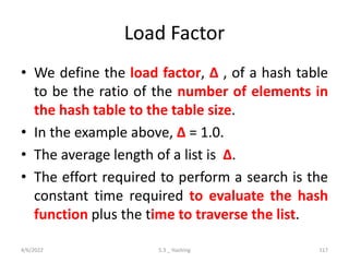
![Open Hashing – Insert Routine
• void insert( element_type key, HASH_TABLE H )
• {
• position pos, new_cell;
• LIST L;
• /*1*/ pos = find( key, H );
• /*2*/ if( pos == NULL )
• {
• /*3*/ new_cell = (position) malloc(sizeof(struct list_node));
• /*4*/ if( new_cell == NULL )
• /*5*/ fatal_error("Out of space!!!");
• else
• {
• /*6*/ L = H->the_lists[ hash( key, H->table size ) ];
• /*7*/ new_cell->next = L->next;
• /*8*/ new_cell->element = key; /* Probably need strcpy!! */
• /*9*/ L->next = new_cell;
• }
• }
• }
4/6/2022 5.3 _ Hashing 115](https://image.slidesharecdn.com/unit5complete-211228094735/85/Searching-Sorting-and-Hashing-Techniques-115-320.jpg)
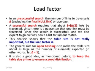

![Closed hashing – Initialization
• HASH_TABLE initialize_table( unsigned int table_size )
• {
• HASH_TABLE H;
• int i;
• /*1*/ if( table_size < MIN_TABLE_SIZE )
• {
• /*2*/ error("Table size too small");
• /*3*/ return NULL;
• }
• /* Allocate table */
• /*4*/ H = (HASH_TABLE) malloc( sizeof ( struct hash_tbl ) );
• /*5*/ if( H == NULL )
• /*6*/ fatal_error("Out of space!!!");
• /*7*/ H->table_size = next_prime( table_size );
• /* Allocate cells */
• /*8*/ H->the cells = (cell *) malloc ( sizeof ( cell ) * H->table_size );
• /*9*/ if( H->the_cells == NULL )
• /*10*/ fatal_error("Out of space!!!");
• /*11*/ for(i=0; i<H->table_size; i++ )
• /*12*/ H->the_cells[i].info = empty;
• /*13*/ return H;
• }
4/6/2022 5.3 _ Hashing 127](https://image.slidesharecdn.com/unit5complete-211228094735/85/Searching-Sorting-and-Hashing-Techniques-127-320.jpg)
![Closed hashing – Find Routine with
Quadratic Probing
• position find( element_type key, HASH_TABLE H )
• {
• position i, current_pos;
• /*1*/ i = 0;
• /*2*/ current_pos = hash( key, H->table_size );
• /* Probably need strcmp! */
• /*3*/ while( (H->the_cells[current_pos].element != key ) &&
• (H->the_cells[current_pos].info != empty ) )
• {
• /*4*/ current_pos += 2*(++i) - 1;
• /*5*/ if( current_pos >= H->table_size )
• /*6*/ current_pos -= H->table_size;
• }
• /*7*/ return current_pos;
• }
4/6/2022 5.3 _ Hashing 128](https://image.slidesharecdn.com/unit5complete-211228094735/85/Searching-Sorting-and-Hashing-Techniques-128-320.jpg)
![Closed hashing – Insert Routine with
Quadratic Probing
• void
• insert( element_type key, HASH_TABLE H )
• {
• position pos;
• pos = find( key, H );
• if( H->the_cells[pos].info != legitimate )
• { /* ok to insert here */
• H->the_cells[pos].info = legitimate;
• H->the_cells[pos].element = key;
• /* Probably need strcpy!! */
• }
• }
4/6/2022 5.3 _ Hashing 129](https://image.slidesharecdn.com/unit5complete-211228094735/85/Searching-Sorting-and-Hashing-Techniques-129-320.jpg)


![Rehashing Implementation - Code
HASH_TABLE
rehash( HASH_TABLE H )
{
unsigned int i, old_size;
cell *old_cells;
/*1*/ old_cells = H->the_cells;
/*2*/ old_size = H->table_size;
/* Get a new, empty table */
/*3*/ H = initialize_table( 2*old_size );
/* Scan through old table, reinserting into new */
/*4*/ for( i=0; i<old_size; i++ )
/*5*/ if( old_cells[i].info == legitimate )
/*6*/ insert( old_cells[i].element, H );
/*7*/ free( old_cells );
/*8*/ return H;
}
4/6/2022 5.3 _ Hashing 141](https://image.slidesharecdn.com/unit5complete-211228094735/85/Searching-Sorting-and-Hashing-Techniques-141-320.jpg)


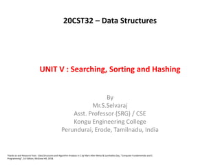
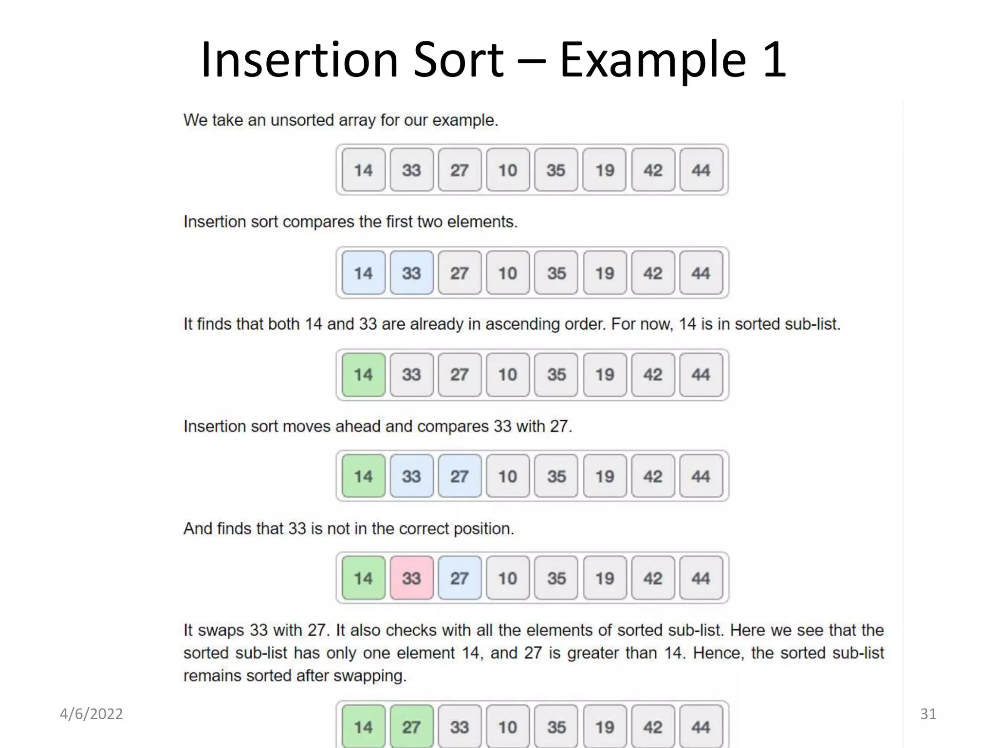
![Insertion Sort - Algorithm
• To sort an array of size n in ascending order:
– 1: Iterate from arr[1] to arr[n] over the array.
– 2: Compare the current element (key) to its
predecessor.
– 3: If the key element is smaller than its
predecessor, compare it to the elements before.
Move the greater elements one position up to
make space for the swapped element.
4/6/2022 5.2 _ Sorting 30](https://image.slidesharecdn.com/unit5complete-211228094735/75/Searching-Sorting-and-Hashing-Techniques-30-2048.jpg)


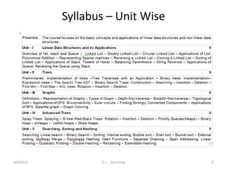
![Quick Sort – Algorithm(Pivot)
• Step 1 - Consider the first element of the list as pivot (i.e., Element at first
position in the list).
• Step 2 - Define two variables i and j. Set i and j to first and last elements of
the list respectively.
• Step 3 - Increment i until list[i] > pivot then stop.
• Step 4 - Decrement j until list[j] < pivot then stop.
• Step 5 - If i < j then exchange list[i] and list[j].
• Step 6 - Repeat steps 3,4 & 5 until i > j.
• Step 7 - Exchange the pivot element with list[j] element.
4/6/2022 5.2 _ Sorting 48](https://image.slidesharecdn.com/unit5complete-211228094735/75/Searching-Sorting-and-Hashing-Techniques-48-2048.jpg)


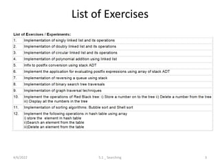
![Open hashing – Initialization
• HASH_TABLE initialize_table( unsigned int table_size )
• {
• HASH_TABLE H;
• int i;
• /*1*/ if( table size < MIN_TABLE_SIZE )
• {
• /*2*/ error("Table size too small");
• /*3*/ return NULL;
• }
• /* Allocate table */
• /*4*/ H = (HASH_TABLE) malloc ( sizeof (struct hash_tbl) );
• /*5*/ if( H == NULL )
• /*6*/ fatal_error("Out of space!!!");
• /*7*/ H->table_size = next_prime( table_size );
• /* Allocate list pointers */
• /*8*/ H->the_lists = (position *) malloc( sizeof (LIST) * H->table_size );
• /*9*/ if( H->the_lists == NULL )
• /*10*/ fatal_error("Out of space!!!");
• /* Allocate list headers */
• /*11*/ for(i=0; i<H->table_size; i++ )
• {
• /*12*/ H->the_lists[i] = (LIST) malloc( sizeof (struct list_node) );
• /*13*/ if( H->the_lists[i] == NULL )
• /*14*/ fatal_error("Out of space!!!");
• else
• /*15*/ H->the_lists[i]->next = NULL;
• }
• /*16*/ return H;
• }
4/6/2022 5.3 _ Hashing 113](https://image.slidesharecdn.com/unit5complete-211228094735/75/Searching-Sorting-and-Hashing-Techniques-113-2048.jpg)
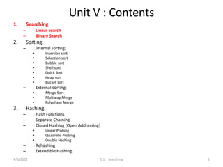
![Open Hashing – Find Routine
• position find( element_type key, HASH_TABLE H )
• {
• position p;
• LIST L;
• /*1*/ L = H->the_lists[ hash( key, H->table_size) ];
• /*2*/ p = L->next;
• /*3*/ while( (p != NULL) && (p->element != key) )
• /* Probably need strcmp!! */
• /*4*/ p = p->next;
• /*5*/ return p;
• }
4/6/2022 5.3 _ Hashing 114](https://image.slidesharecdn.com/unit5complete-211228094735/75/Searching-Sorting-and-Hashing-Techniques-114-2048.jpg)
![Open Hashing – Insert Routine
• void insert( element_type key, HASH_TABLE H )
• {
• position pos, new_cell;
• LIST L;
• /*1*/ pos = find( key, H );
• /*2*/ if( pos == NULL )
• {
• /*3*/ new_cell = (position) malloc(sizeof(struct list_node));
• /*4*/ if( new_cell == NULL )
• /*5*/ fatal_error("Out of space!!!");
• else
• {
• /*6*/ L = H->the_lists[ hash( key, H->table size ) ];
• /*7*/ new_cell->next = L->next;
• /*8*/ new_cell->element = key; /* Probably need strcpy!! */
• /*9*/ L->next = new_cell;
• }
• }
• }
4/6/2022 5.3 _ Hashing 115](https://image.slidesharecdn.com/unit5complete-211228094735/75/Searching-Sorting-and-Hashing-Techniques-115-2048.jpg)


![Closed hashing – Initialization
• HASH_TABLE initialize_table( unsigned int table_size )
• {
• HASH_TABLE H;
• int i;
• /*1*/ if( table_size < MIN_TABLE_SIZE )
• {
• /*2*/ error("Table size too small");
• /*3*/ return NULL;
• }
• /* Allocate table */
• /*4*/ H = (HASH_TABLE) malloc( sizeof ( struct hash_tbl ) );
• /*5*/ if( H == NULL )
• /*6*/ fatal_error("Out of space!!!");
• /*7*/ H->table_size = next_prime( table_size );
• /* Allocate cells */
• /*8*/ H->the cells = (cell *) malloc ( sizeof ( cell ) * H->table_size );
• /*9*/ if( H->the_cells == NULL )
• /*10*/ fatal_error("Out of space!!!");
• /*11*/ for(i=0; i<H->table_size; i++ )
• /*12*/ H->the_cells[i].info = empty;
• /*13*/ return H;
• }
4/6/2022 5.3 _ Hashing 127](https://image.slidesharecdn.com/unit5complete-211228094735/75/Searching-Sorting-and-Hashing-Techniques-127-2048.jpg)
![Closed hashing – Find Routine with
Quadratic Probing
• position find( element_type key, HASH_TABLE H )
• {
• position i, current_pos;
• /*1*/ i = 0;
• /*2*/ current_pos = hash( key, H->table_size );
• /* Probably need strcmp! */
• /*3*/ while( (H->the_cells[current_pos].element != key ) &&
• (H->the_cells[current_pos].info != empty ) )
• {
• /*4*/ current_pos += 2*(++i) - 1;
• /*5*/ if( current_pos >= H->table_size )
• /*6*/ current_pos -= H->table_size;
• }
• /*7*/ return current_pos;
• }
4/6/2022 5.3 _ Hashing 128](https://image.slidesharecdn.com/unit5complete-211228094735/75/Searching-Sorting-and-Hashing-Techniques-128-2048.jpg)
![Closed hashing – Insert Routine with
Quadratic Probing
• void
• insert( element_type key, HASH_TABLE H )
• {
• position pos;
• pos = find( key, H );
• if( H->the_cells[pos].info != legitimate )
• { /* ok to insert here */
• H->the_cells[pos].info = legitimate;
• H->the_cells[pos].element = key;
• /* Probably need strcpy!! */
• }
• }
4/6/2022 5.3 _ Hashing 129](https://image.slidesharecdn.com/unit5complete-211228094735/75/Searching-Sorting-and-Hashing-Techniques-129-2048.jpg)


![Rehashing Implementation - Code
HASH_TABLE
rehash( HASH_TABLE H )
{
unsigned int i, old_size;
cell *old_cells;
/*1*/ old_cells = H->the_cells;
/*2*/ old_size = H->table_size;
/* Get a new, empty table */
/*3*/ H = initialize_table( 2*old_size );
/* Scan through old table, reinserting into new */
/*4*/ for( i=0; i<old_size; i++ )
/*5*/ if( old_cells[i].info == legitimate )
/*6*/ insert( old_cells[i].element, H );
/*7*/ free( old_cells );
/*8*/ return H;
}
4/6/2022 5.3 _ Hashing 141](https://image.slidesharecdn.com/unit5complete-211228094735/75/Searching-Sorting-and-Hashing-Techniques-141-2048.jpg)


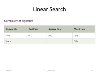
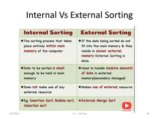
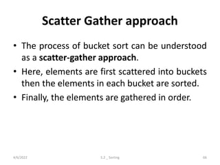
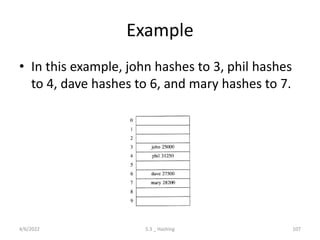
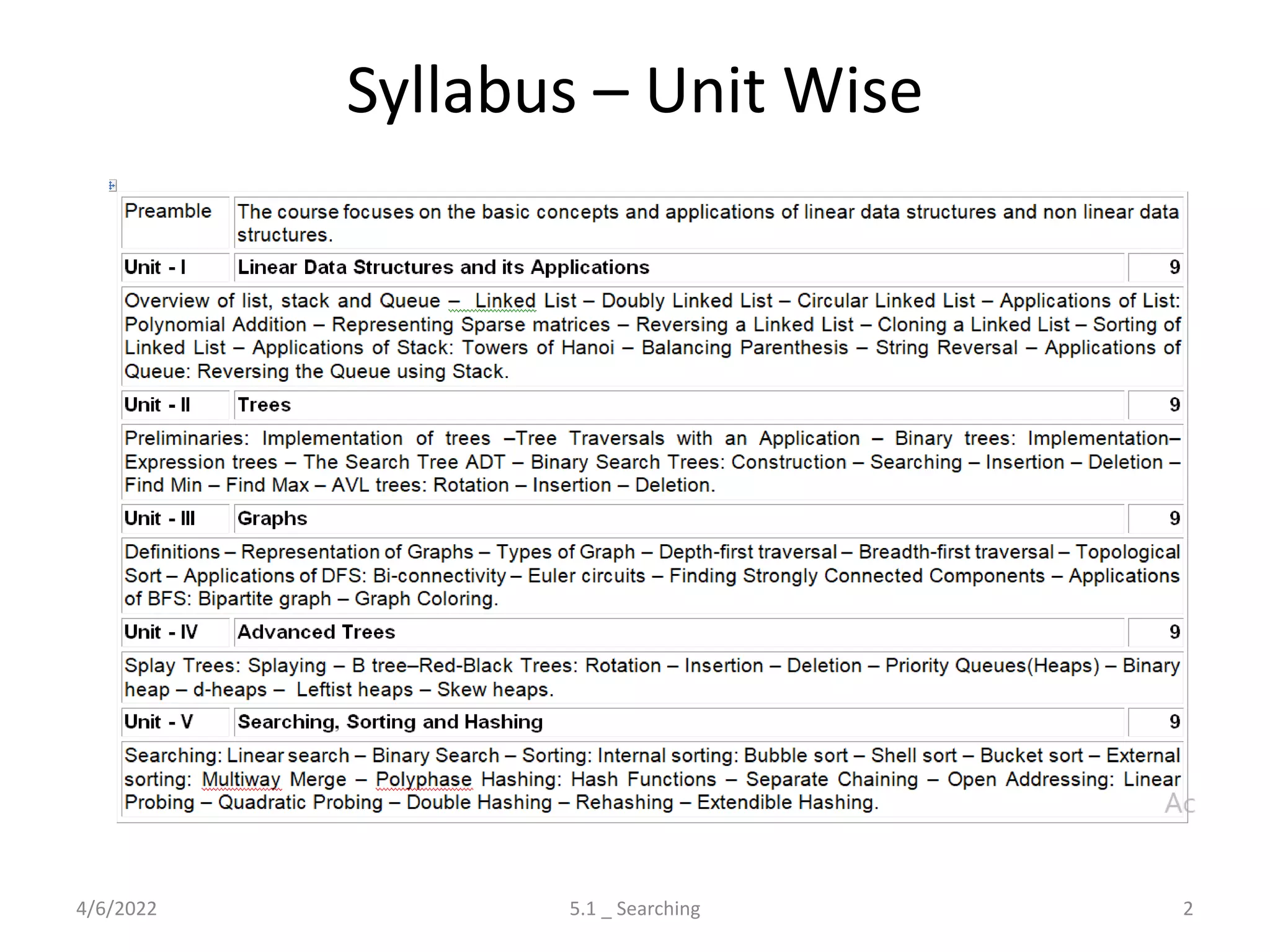
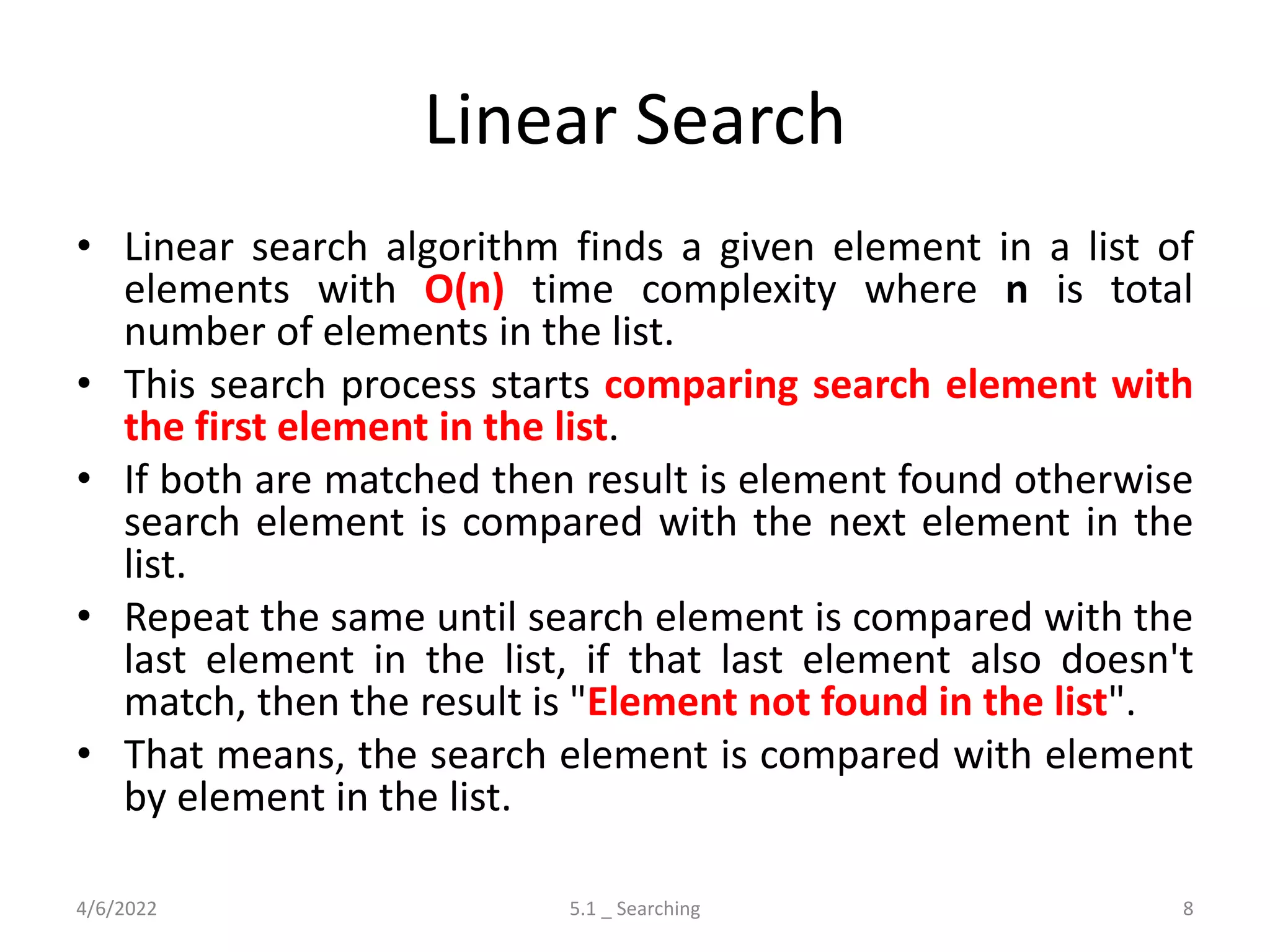
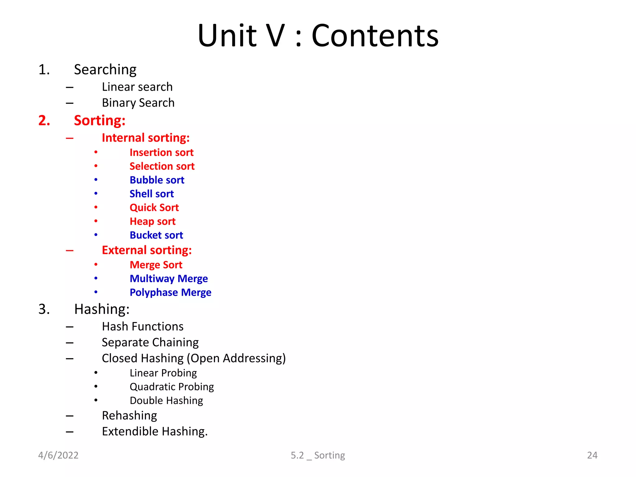
The document outlines Unit V of a data structures course, focusing on searching, sorting, and hashing techniques. It details various searching algorithms such as linear and binary search, alongside multiple sorting methods including insertion, selection, and quick sort, along with their complexities and algorithms. Additionally, it covers hashing methods, emphasizing their significance in data structure operations.
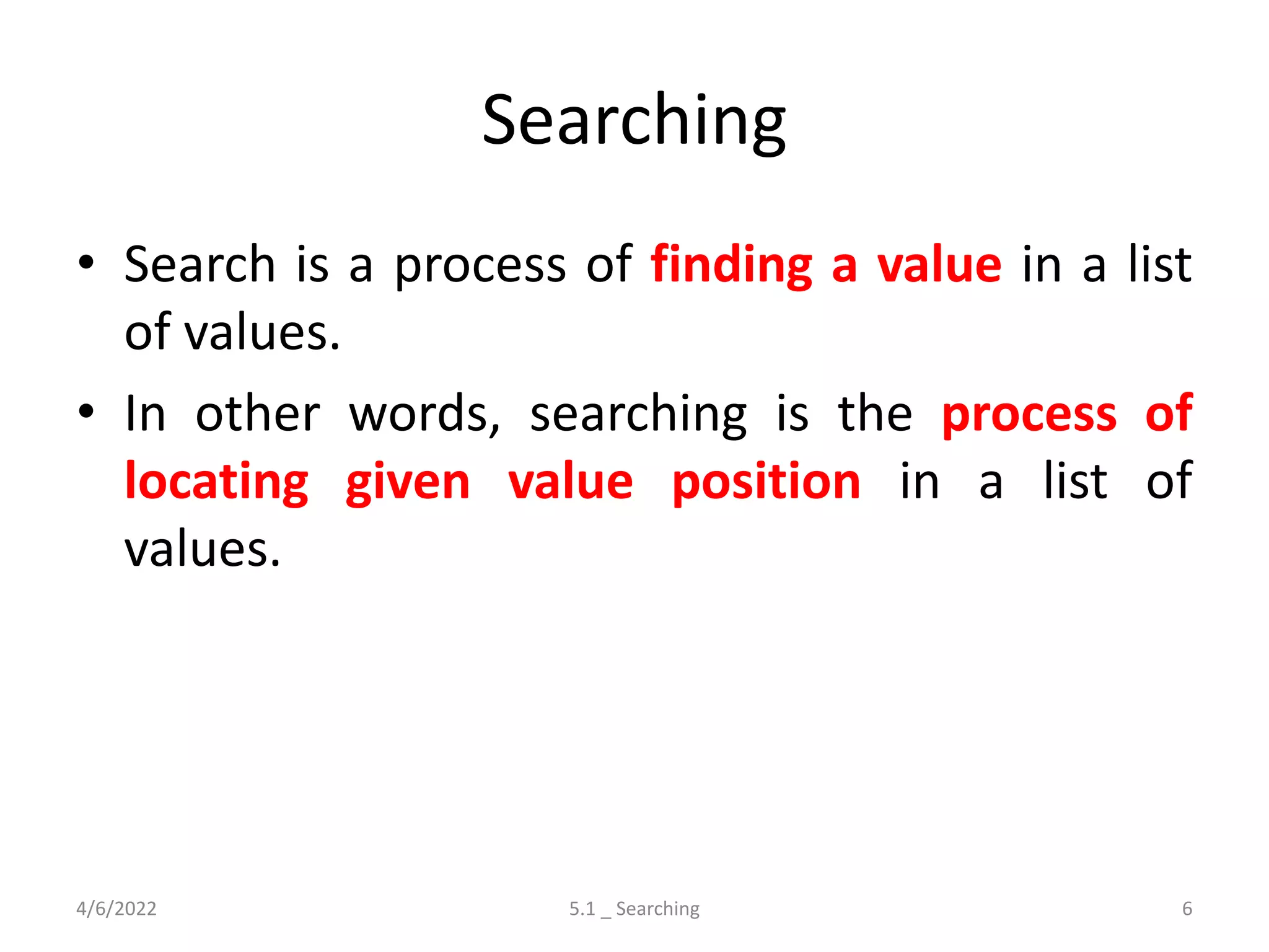
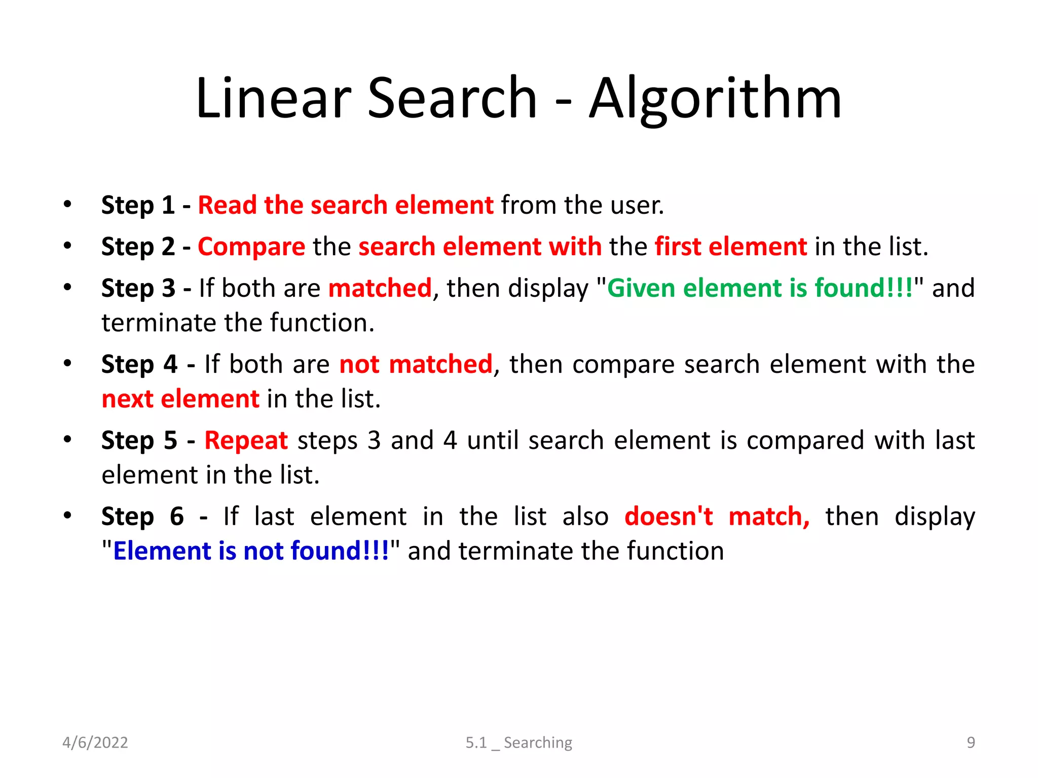
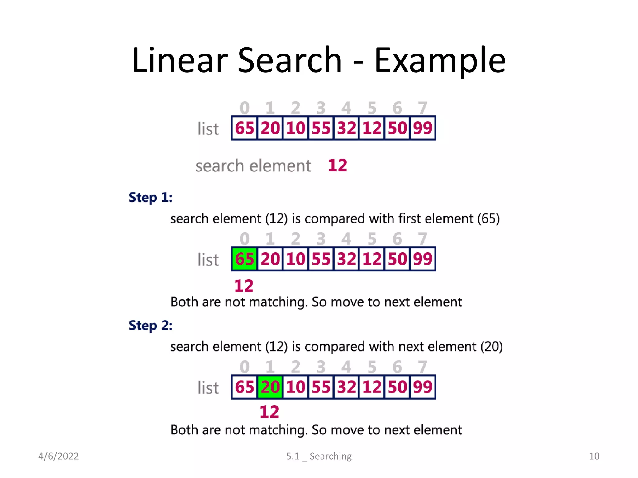
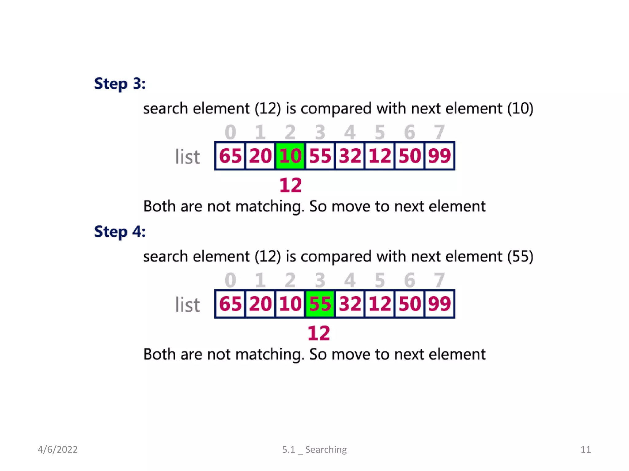
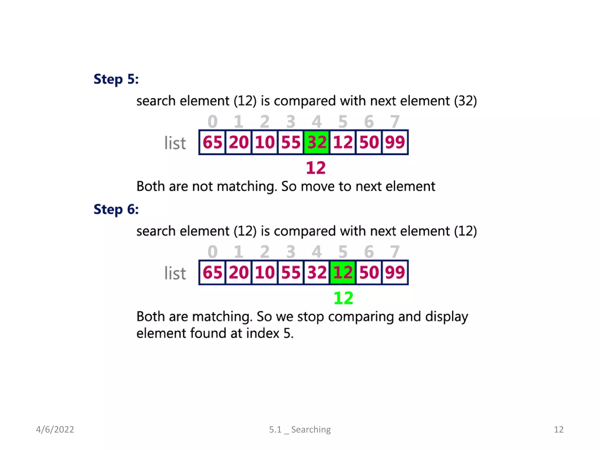
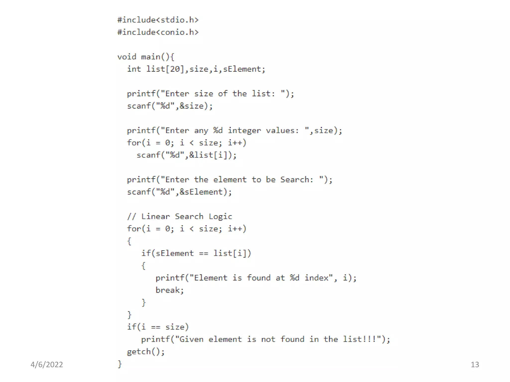
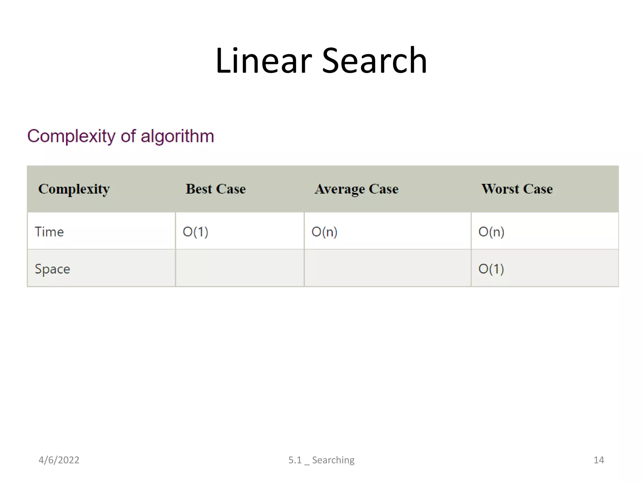
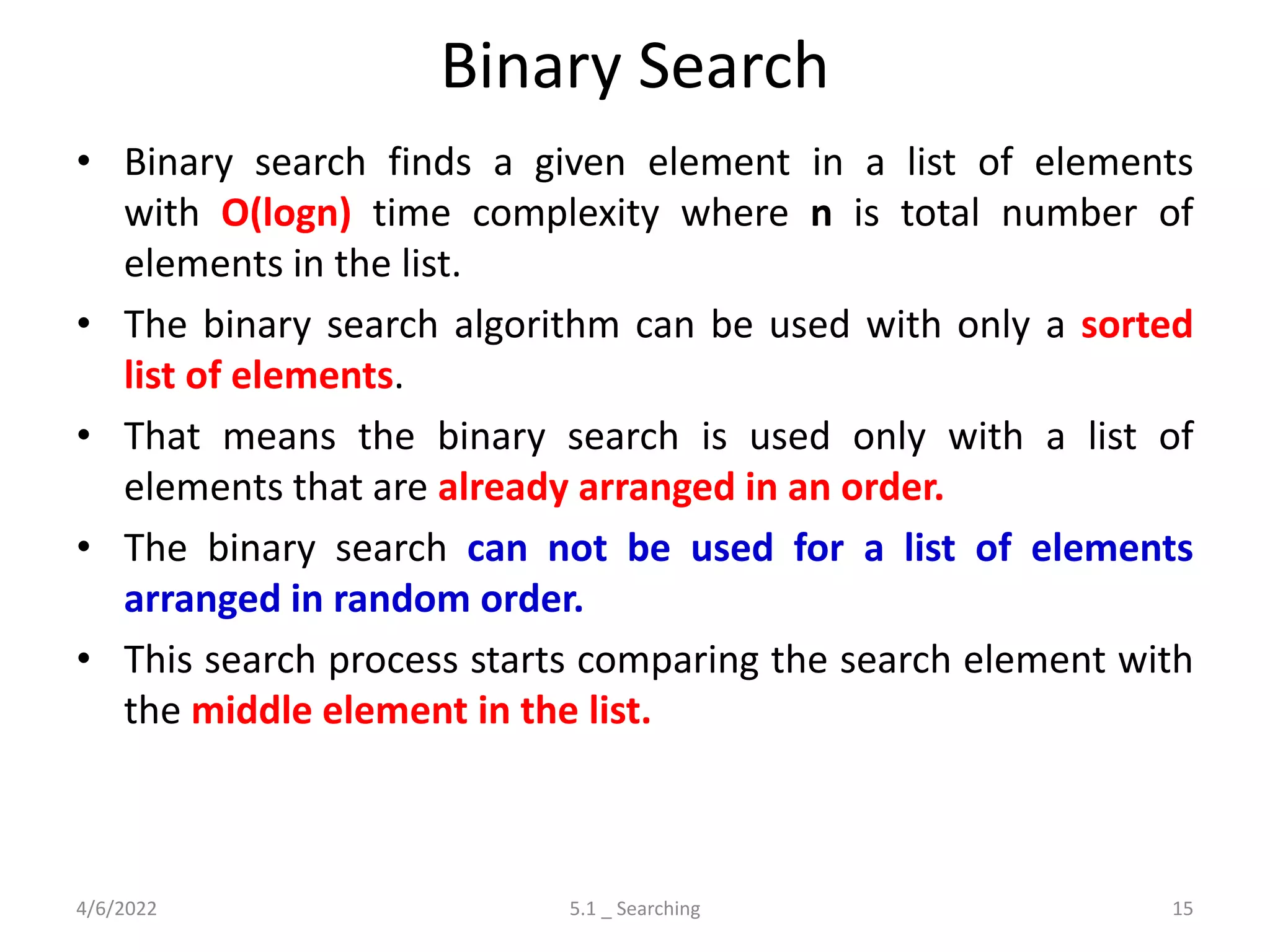
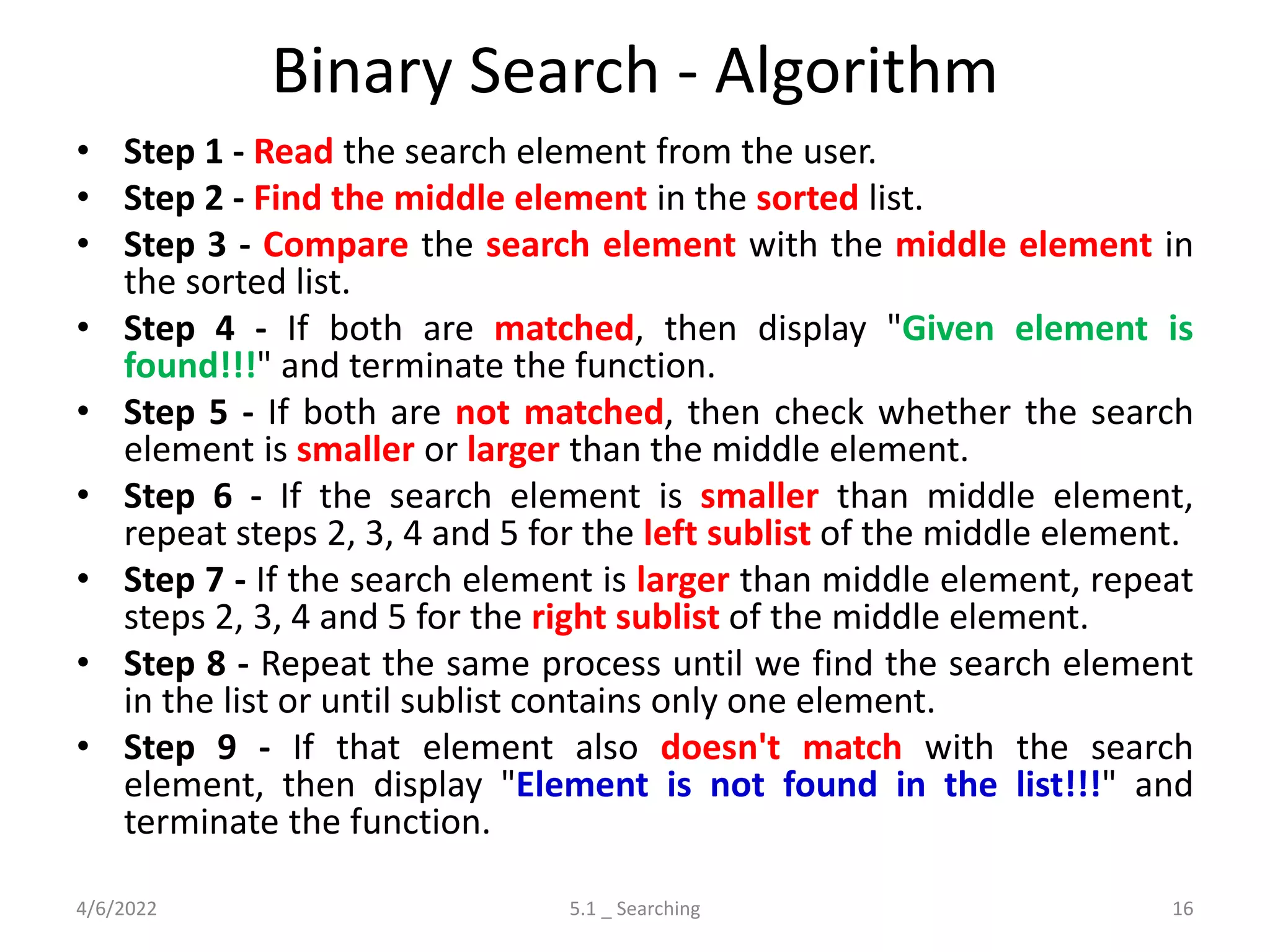
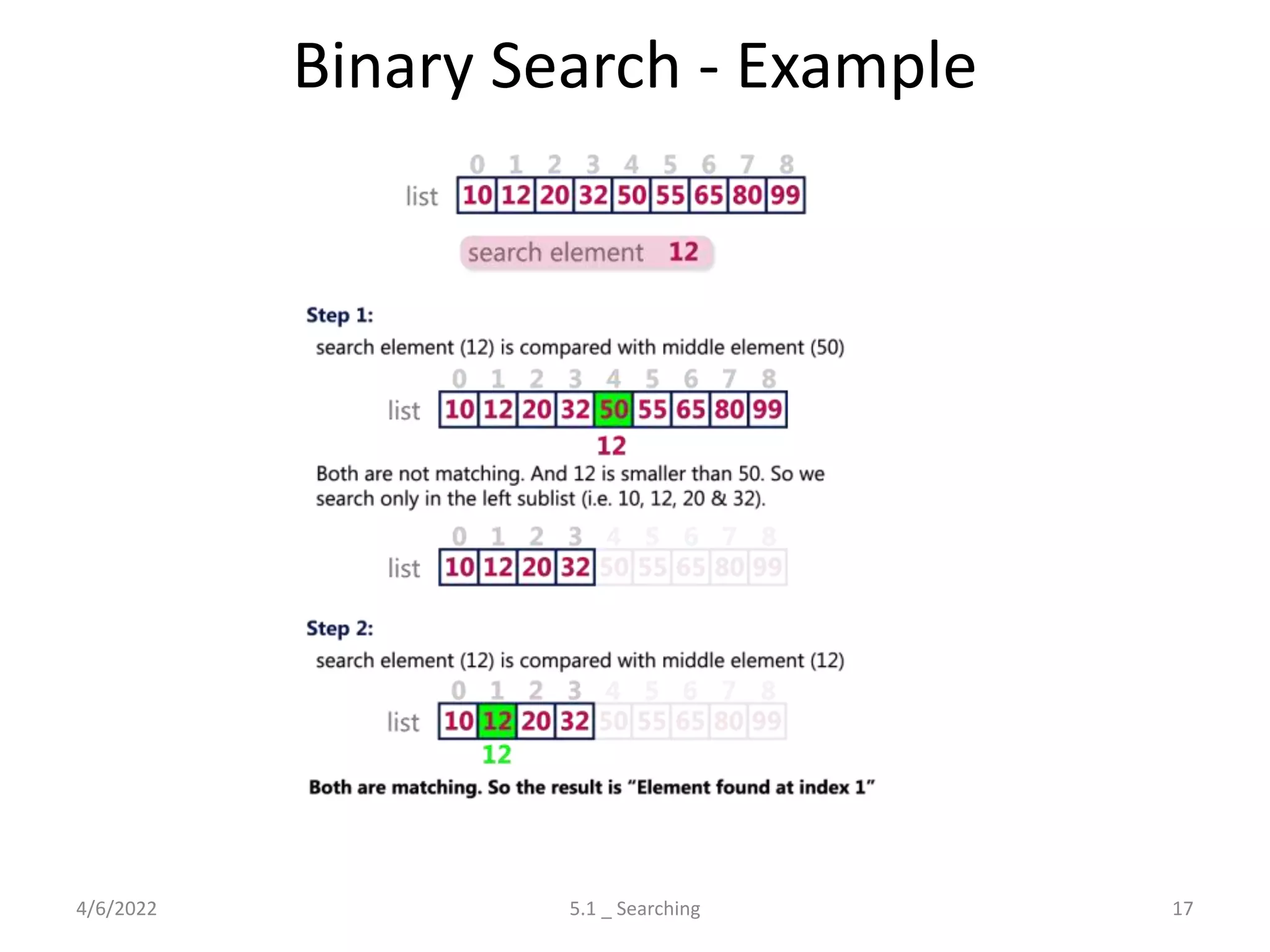
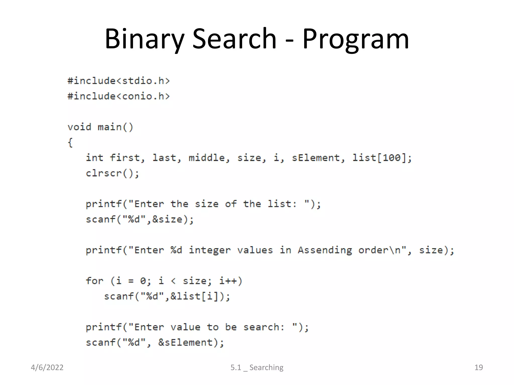
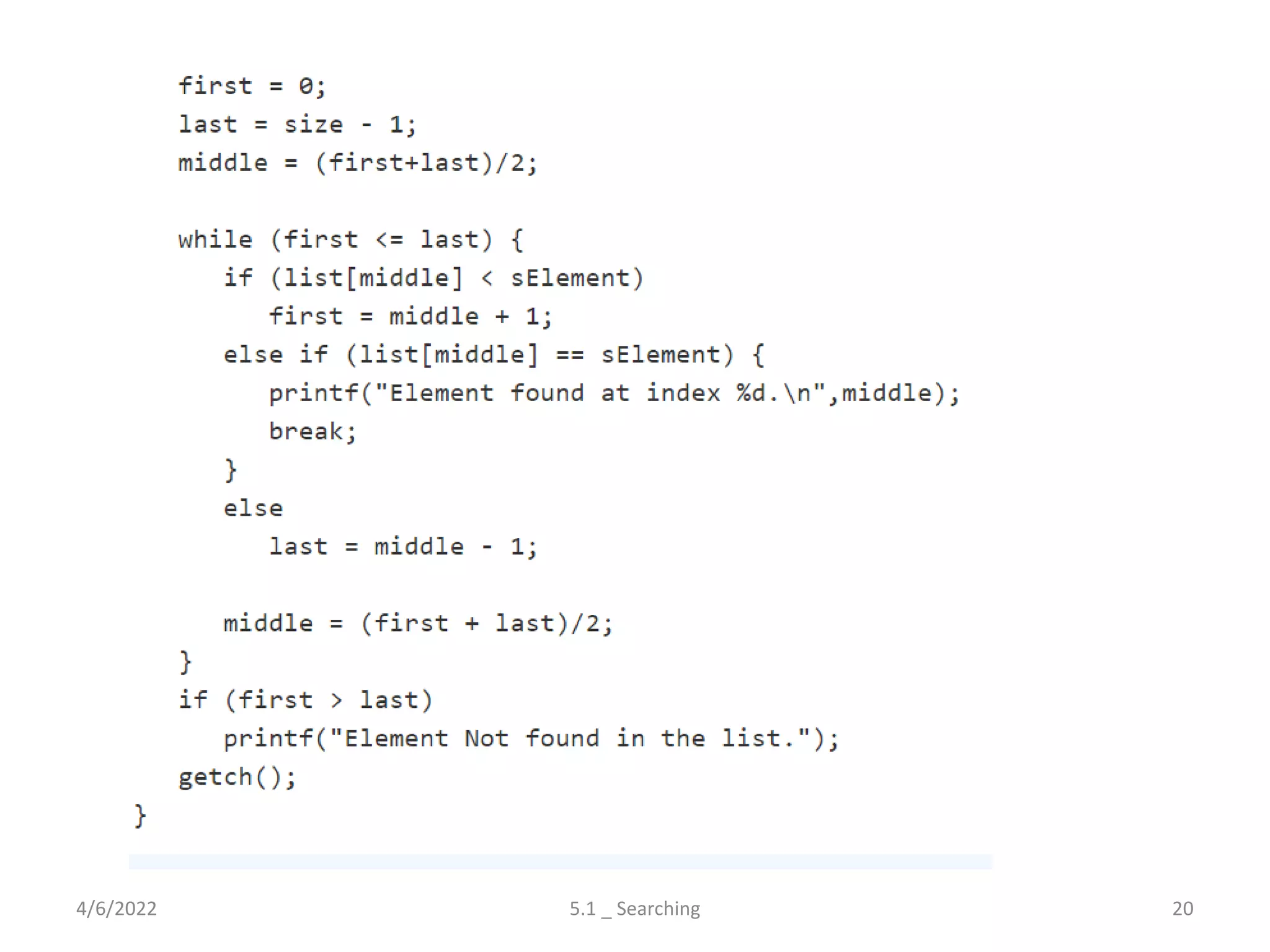
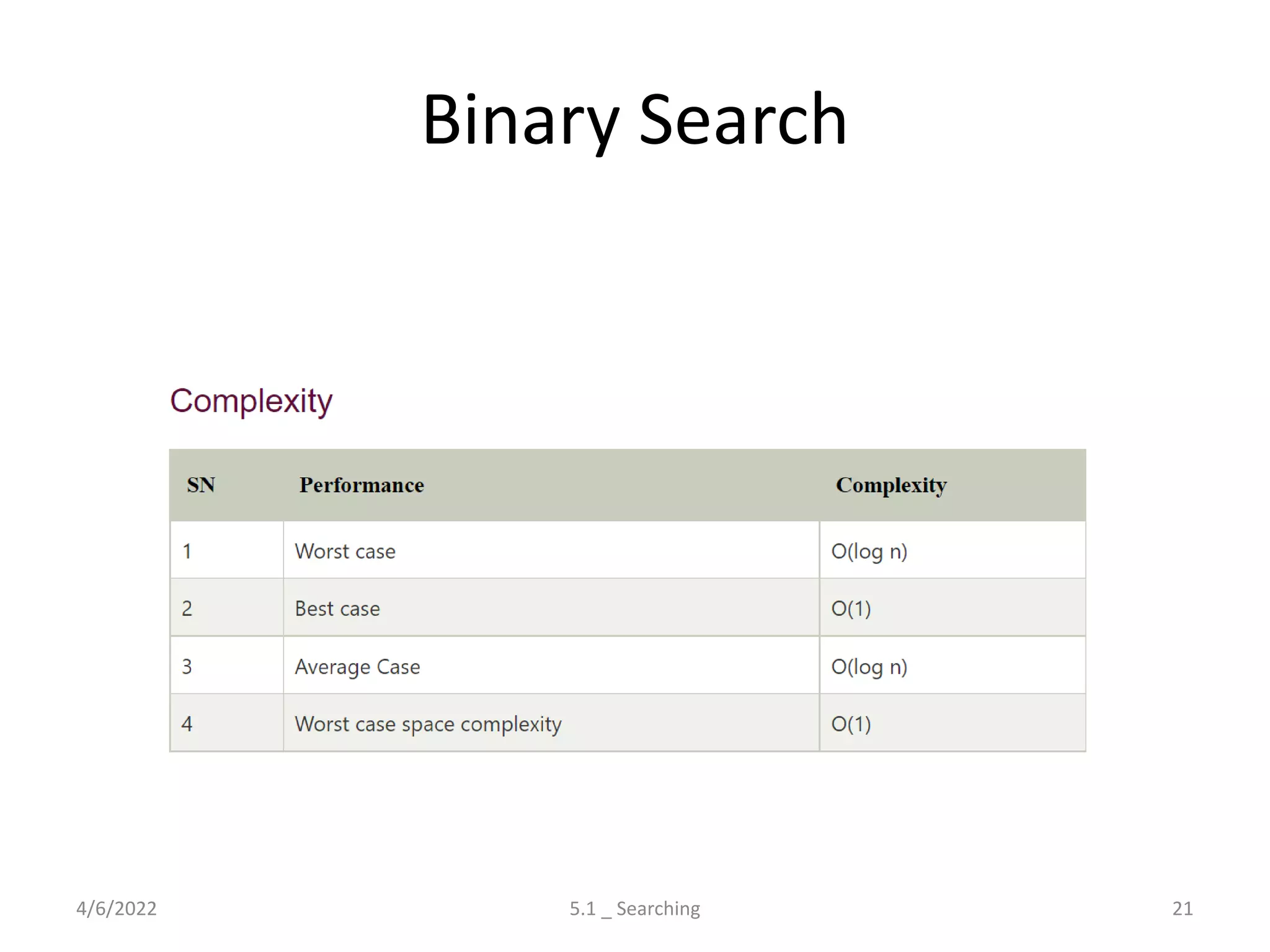
Discusses the process of searching in lists, covering linear and binary search algorithms with their respective properties and complexities.
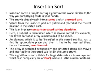
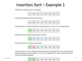
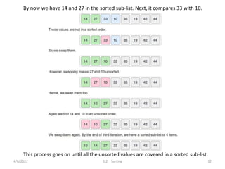
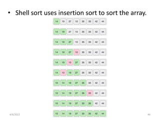
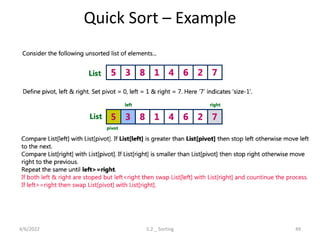
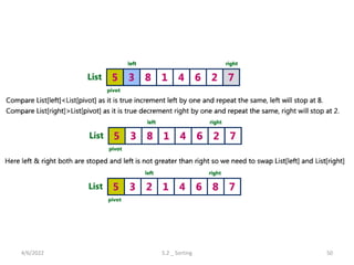
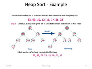
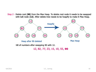
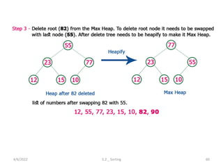
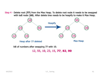
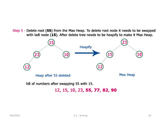
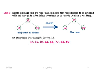
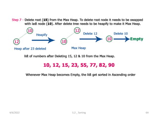
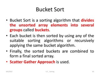
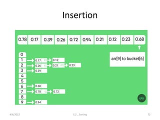
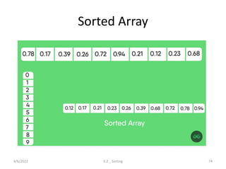
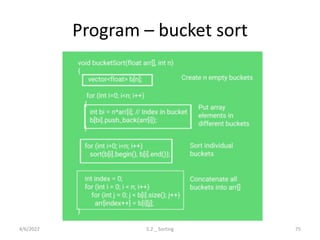
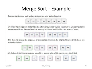
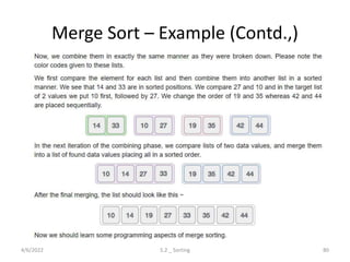
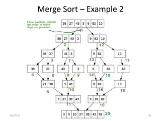
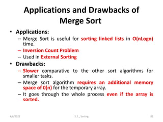
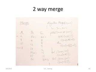
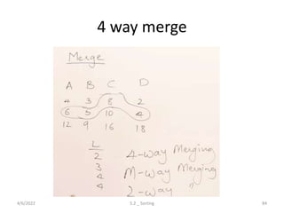
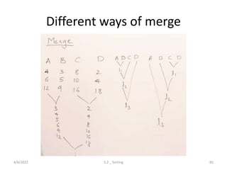
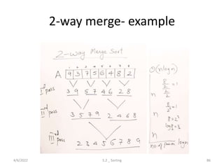
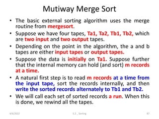
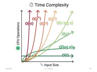
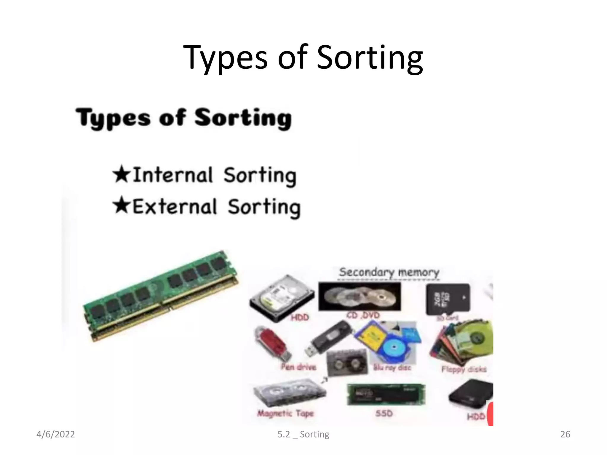
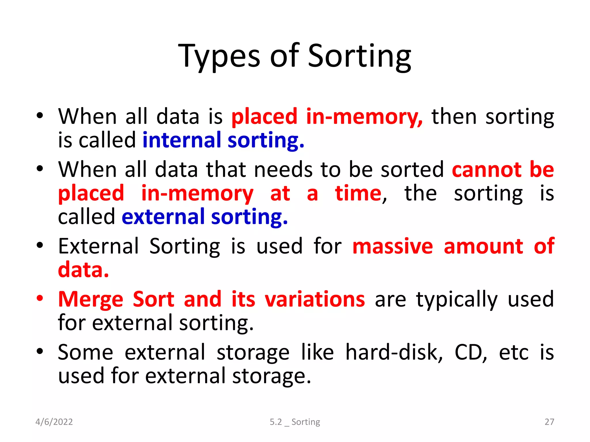
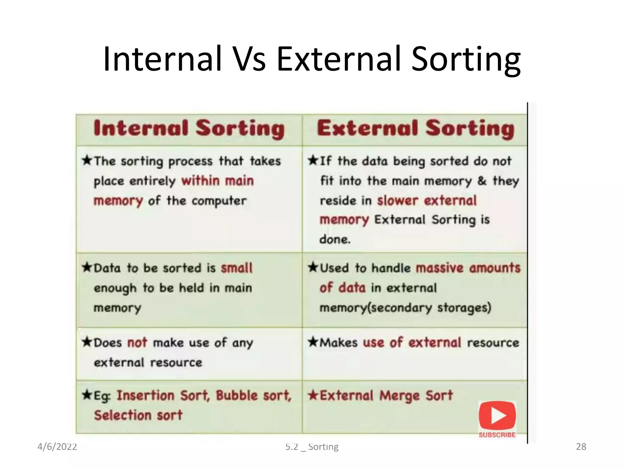
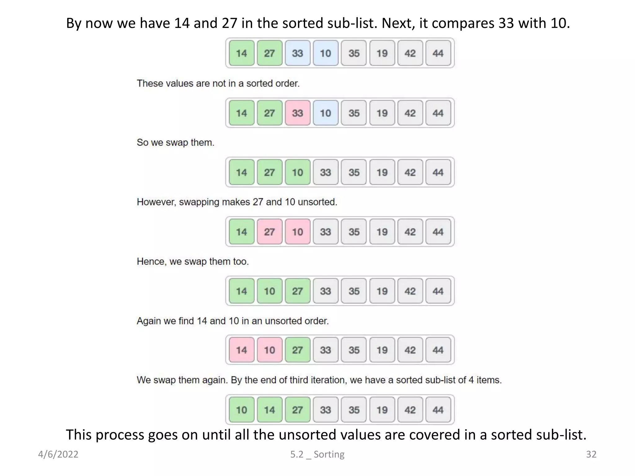
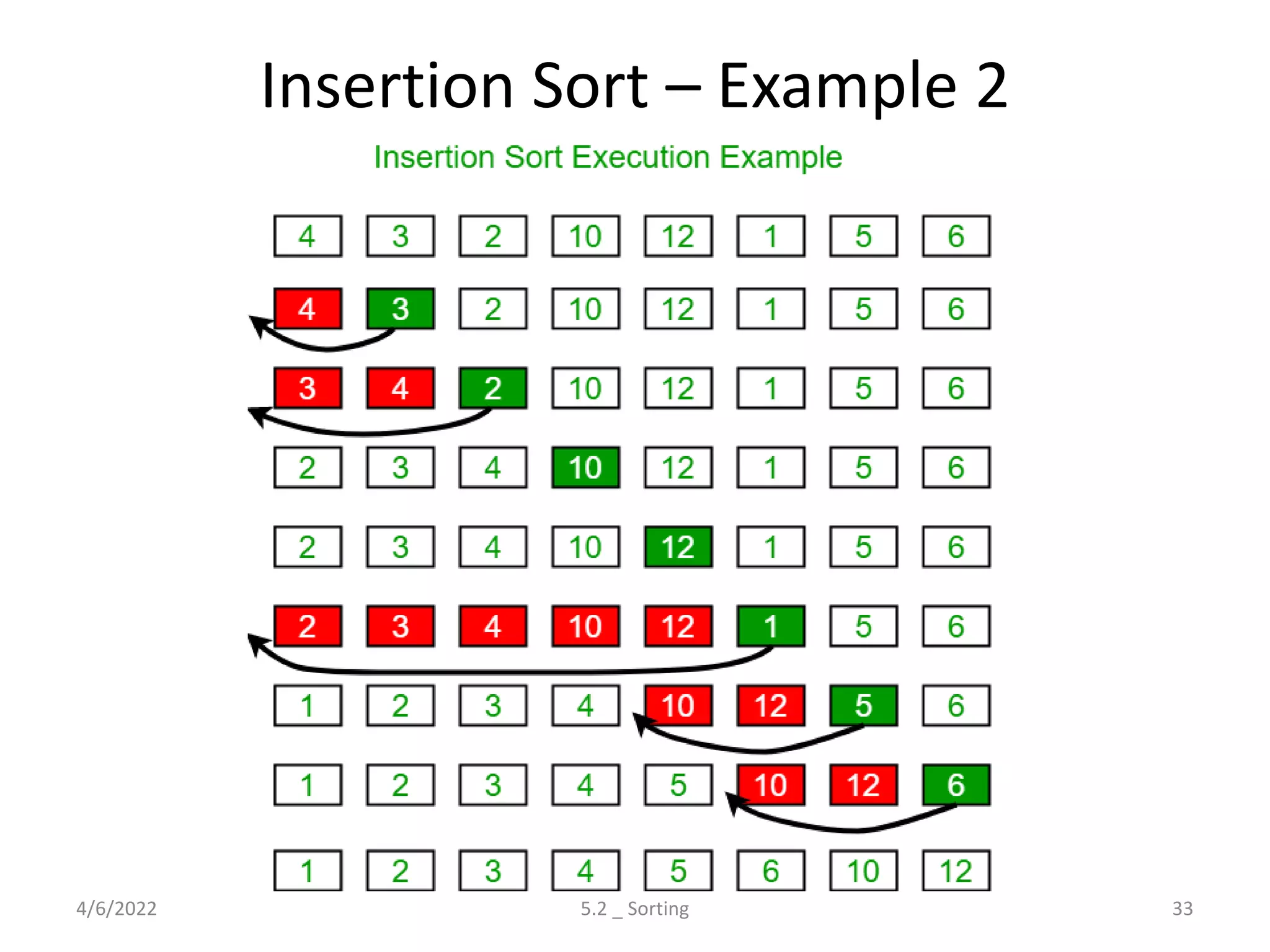
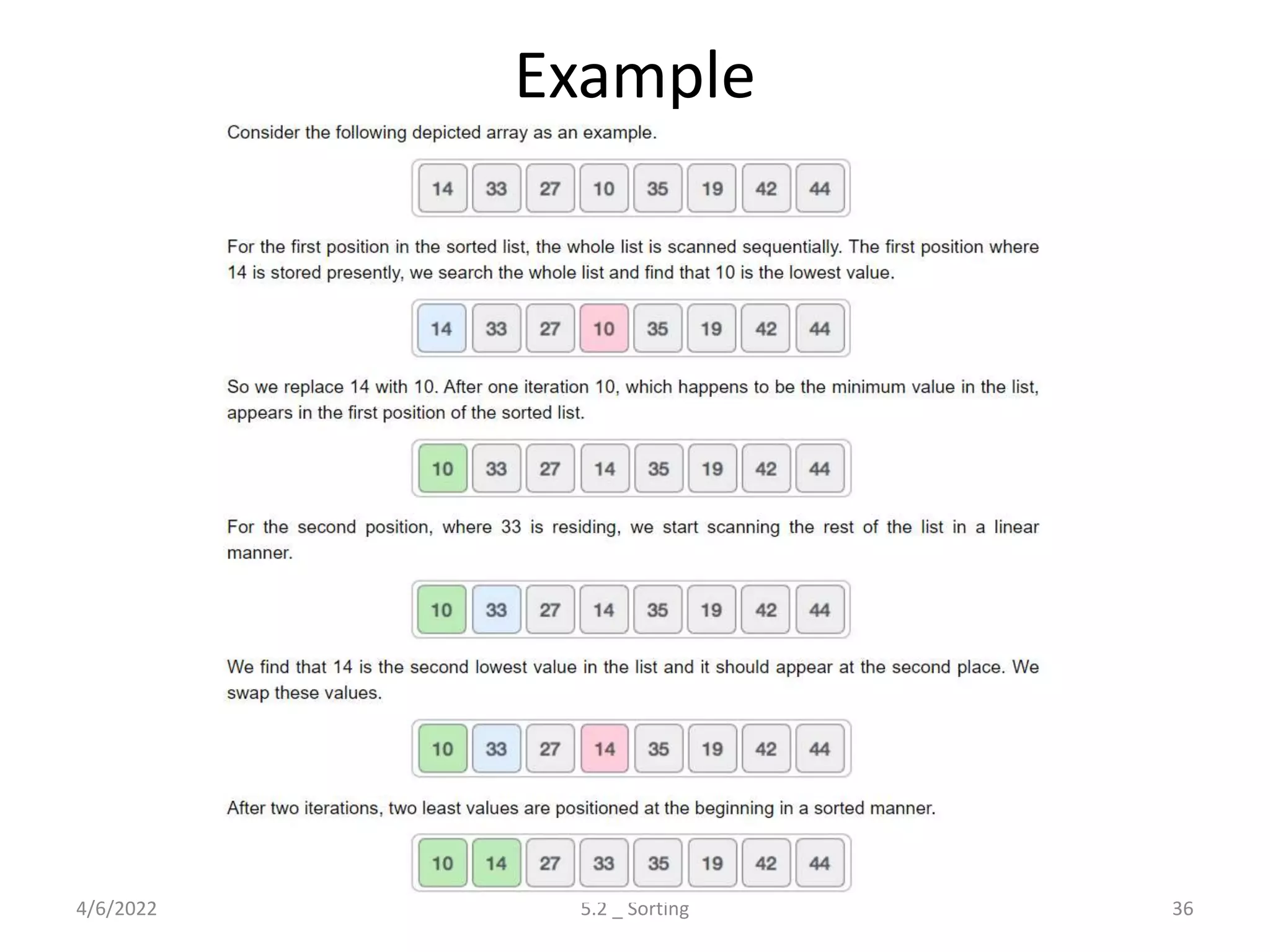
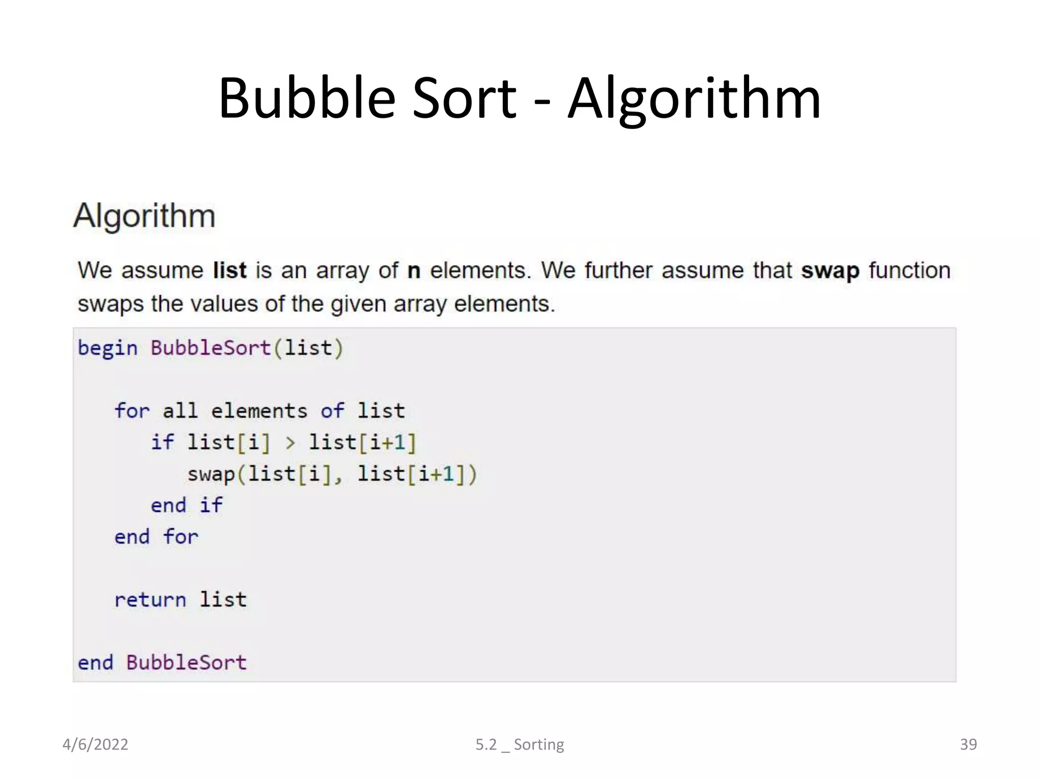
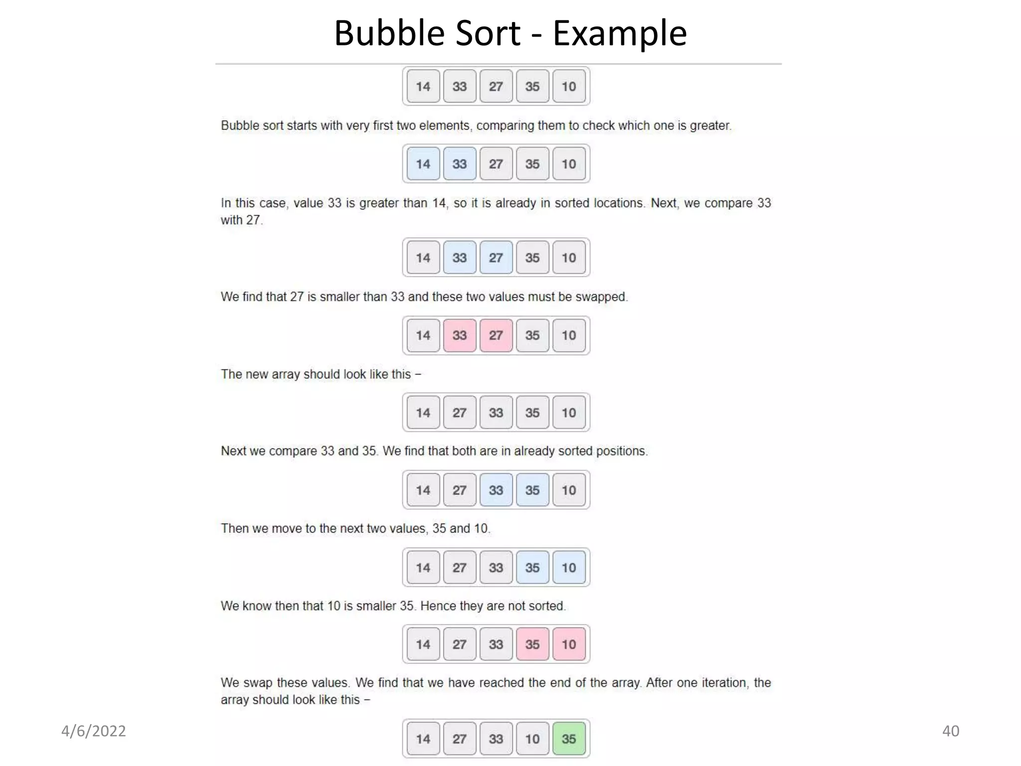
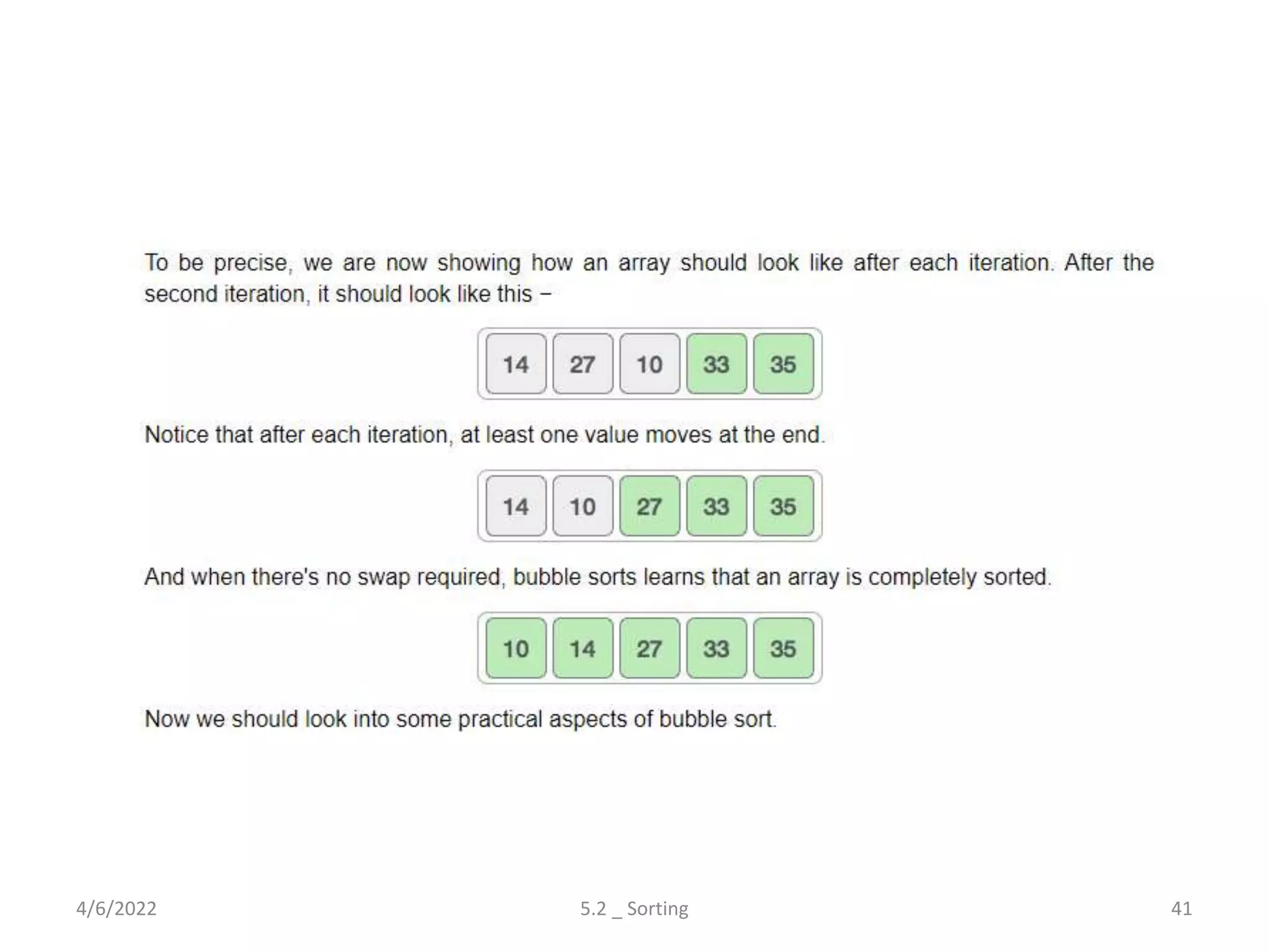
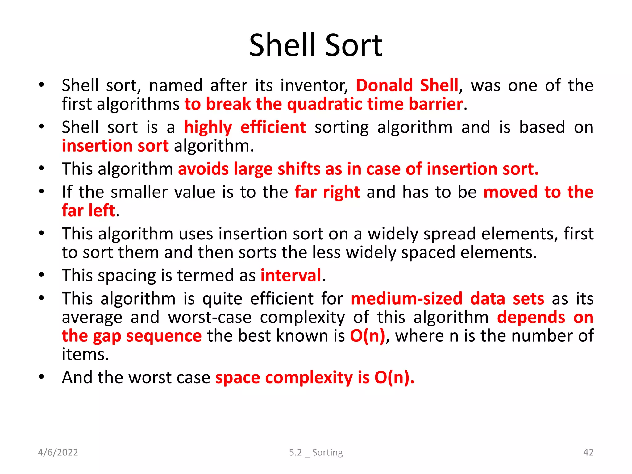
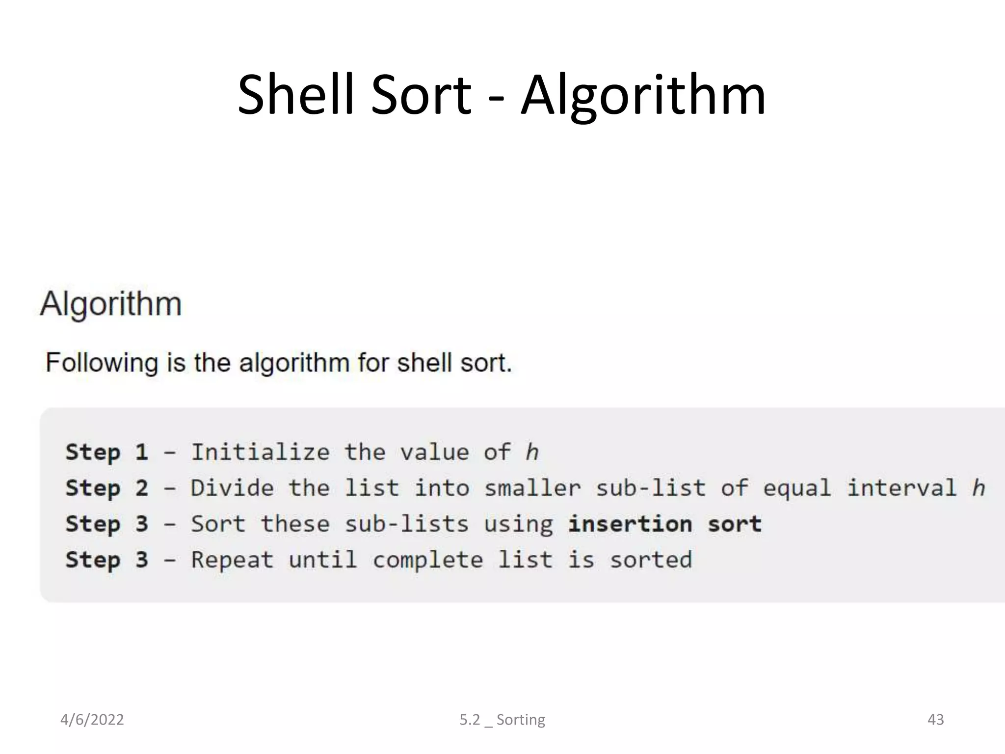
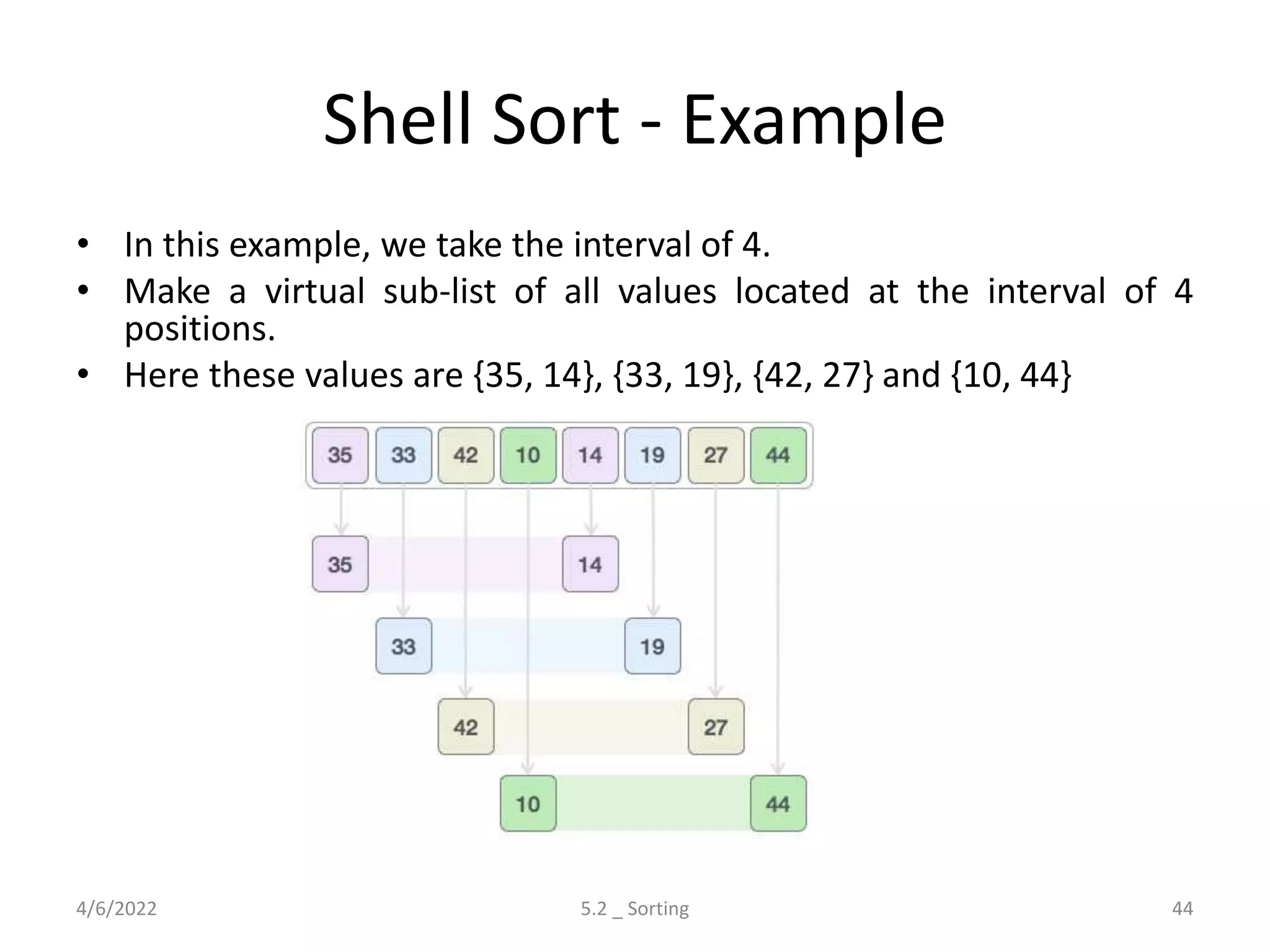
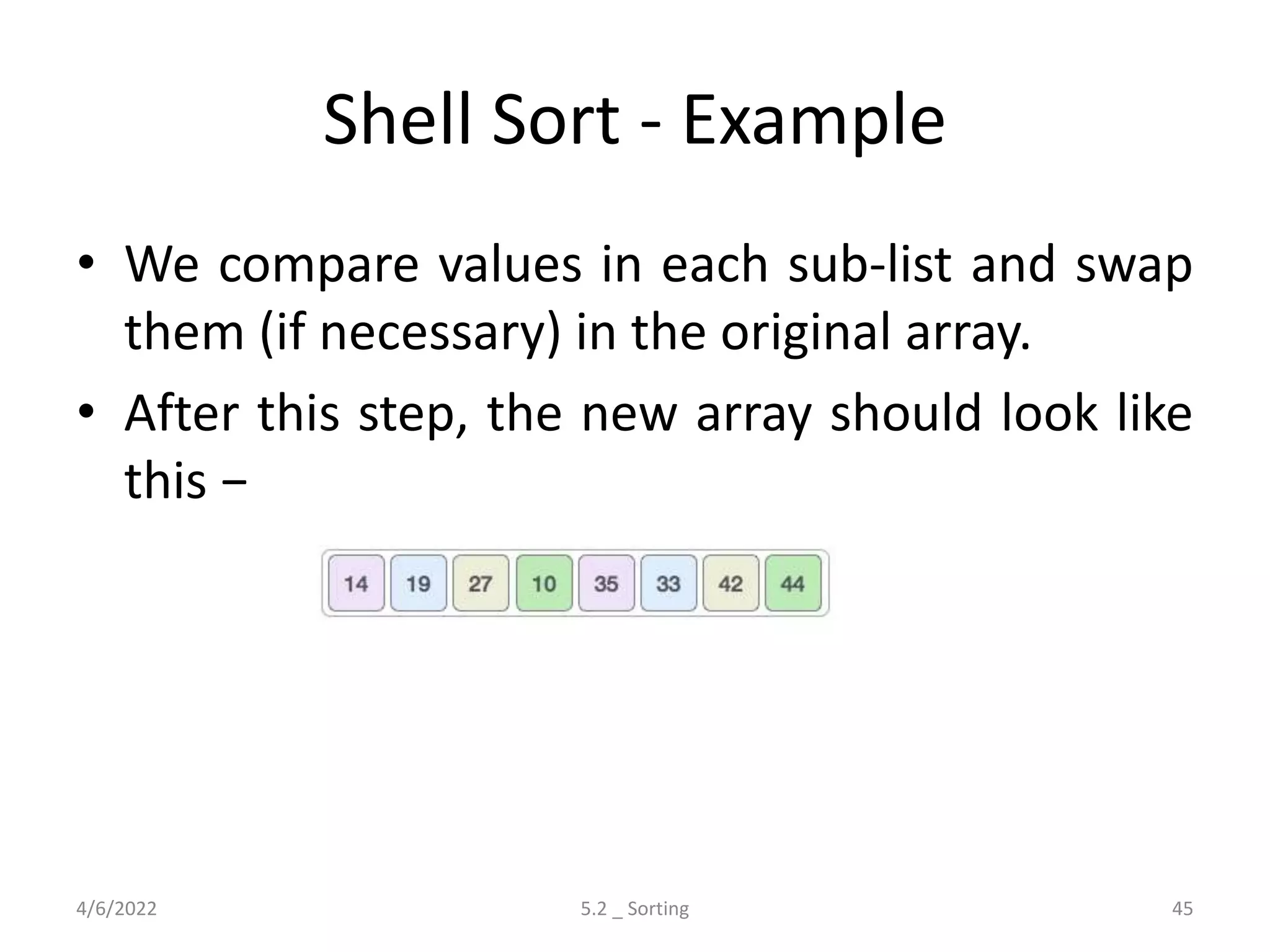
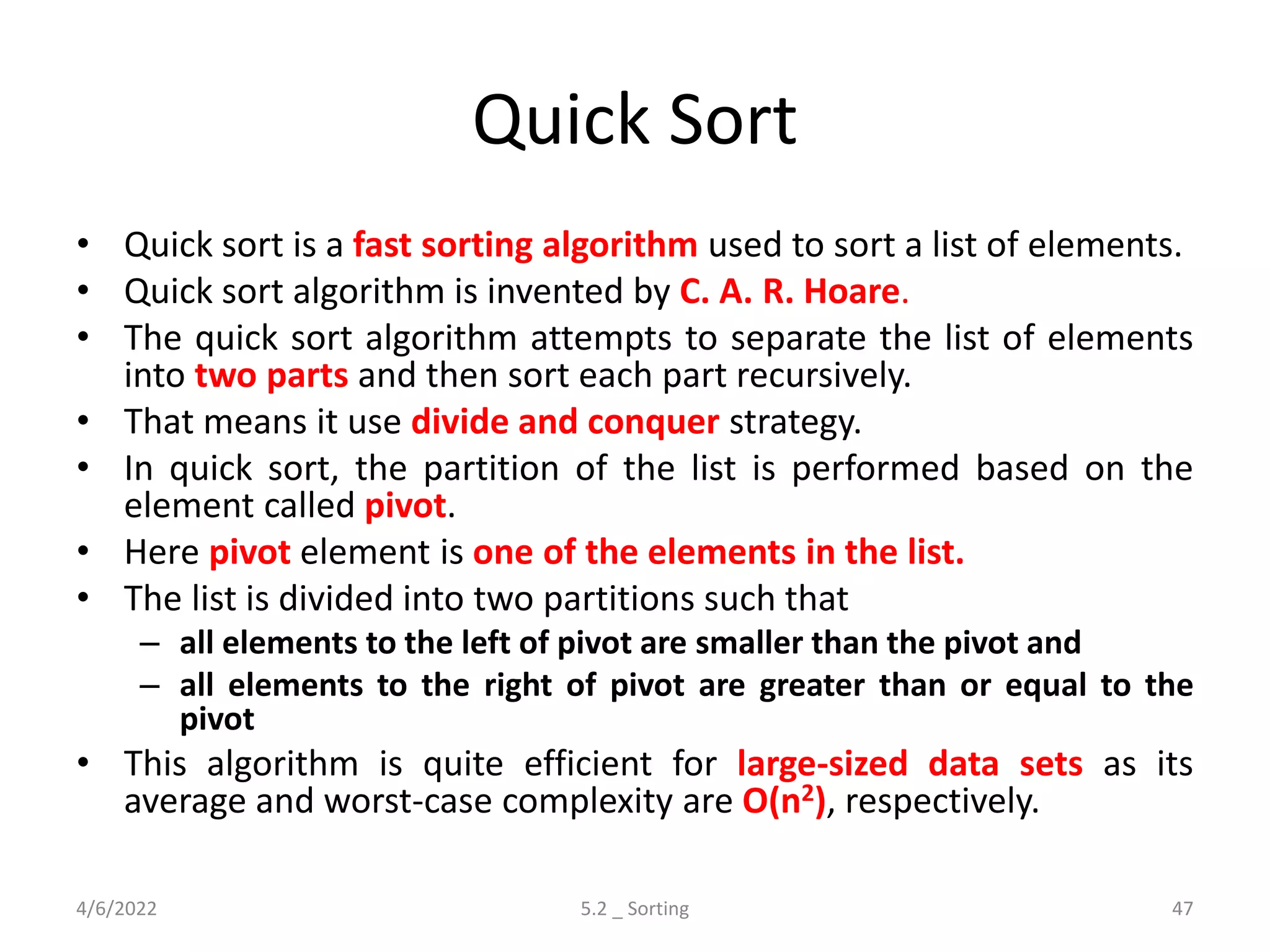
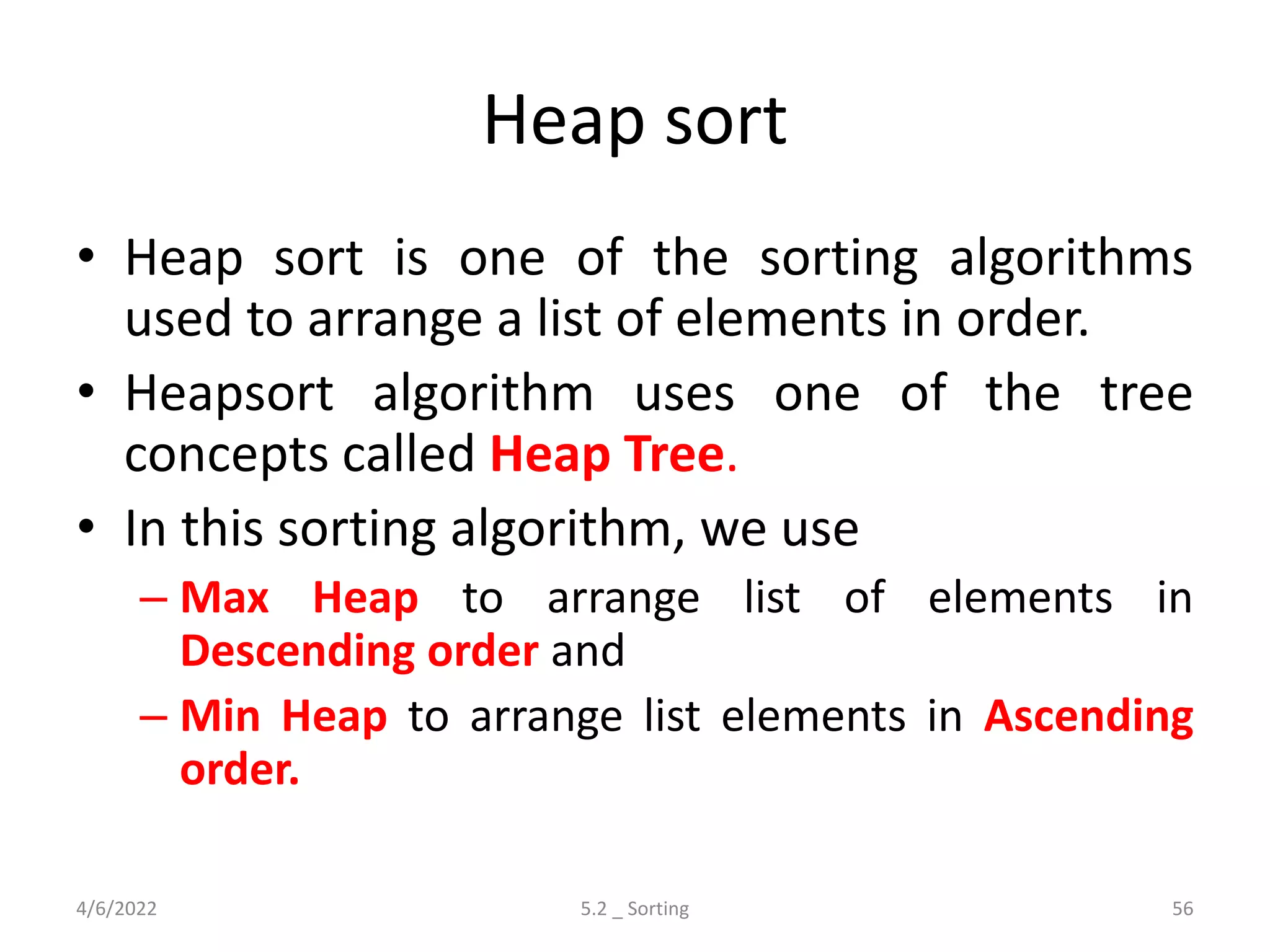
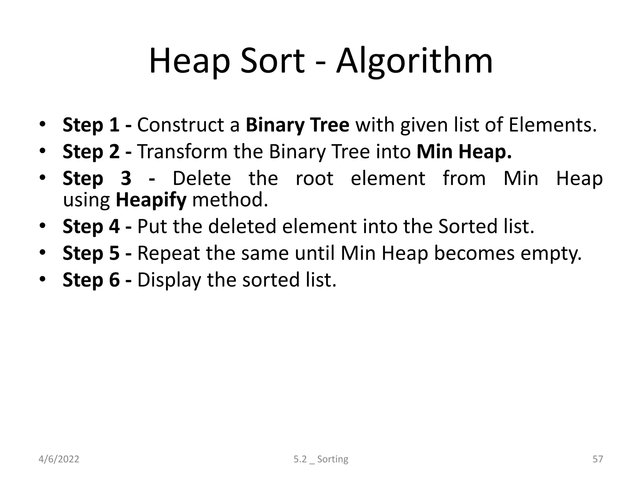
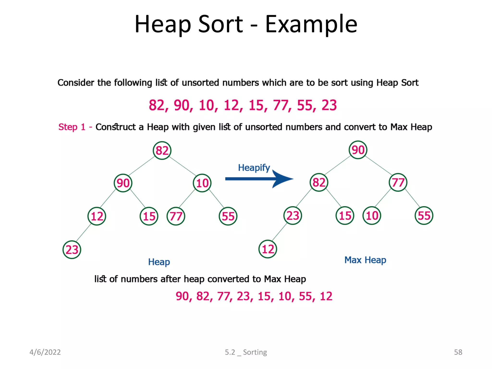
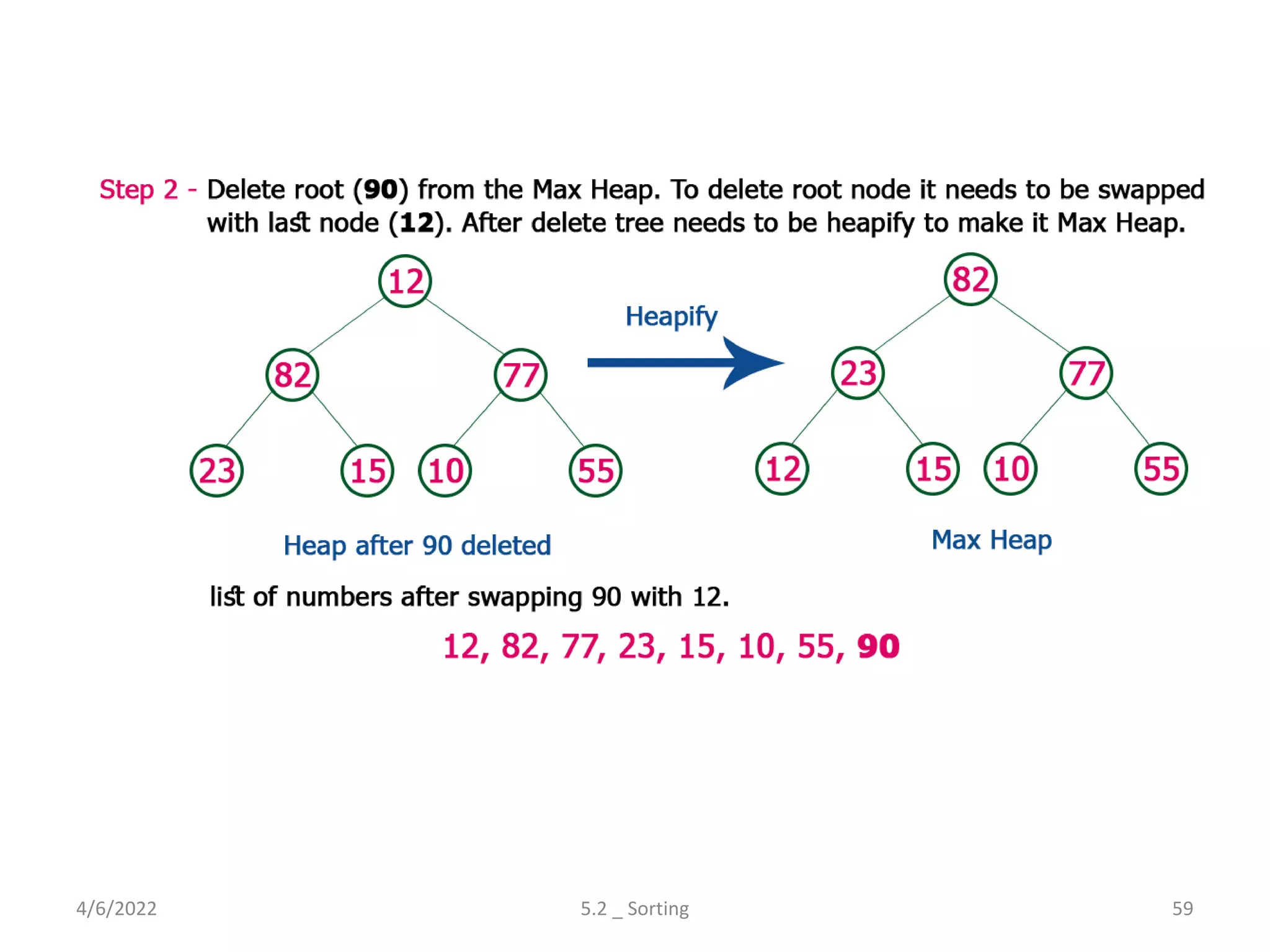
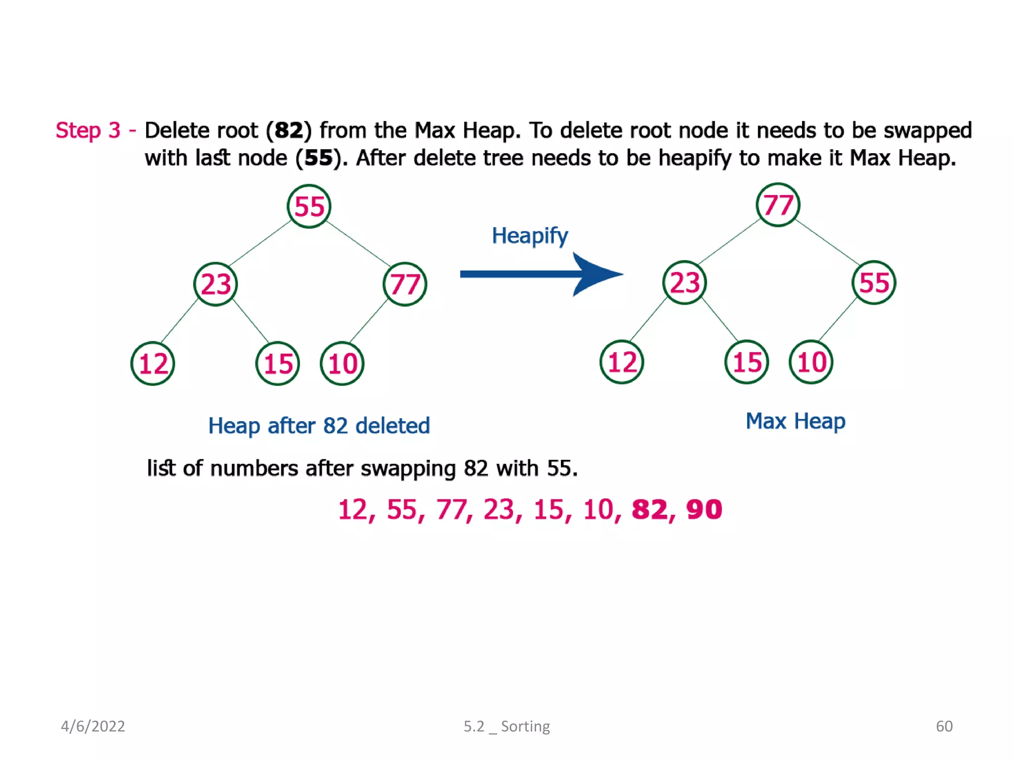
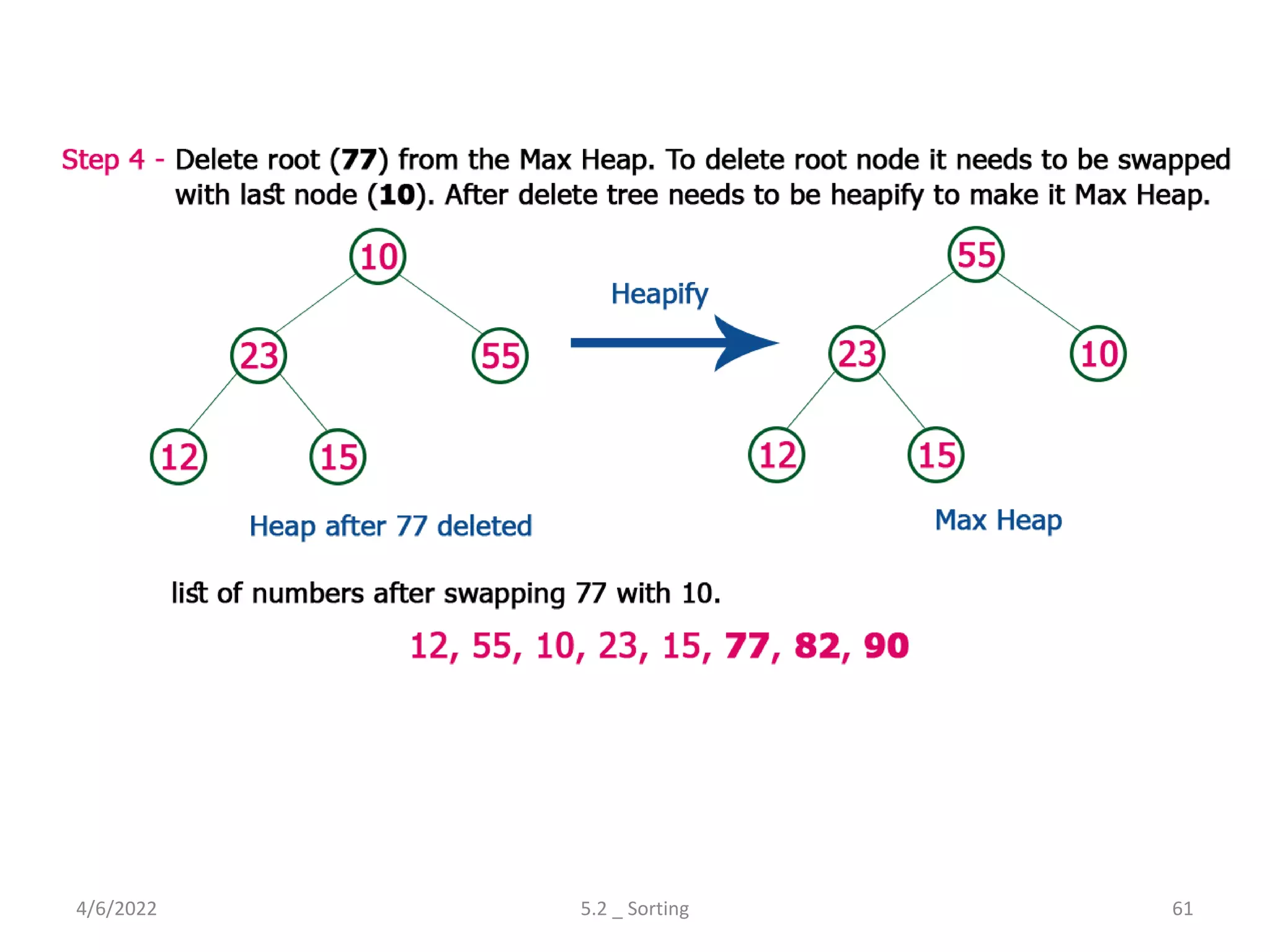
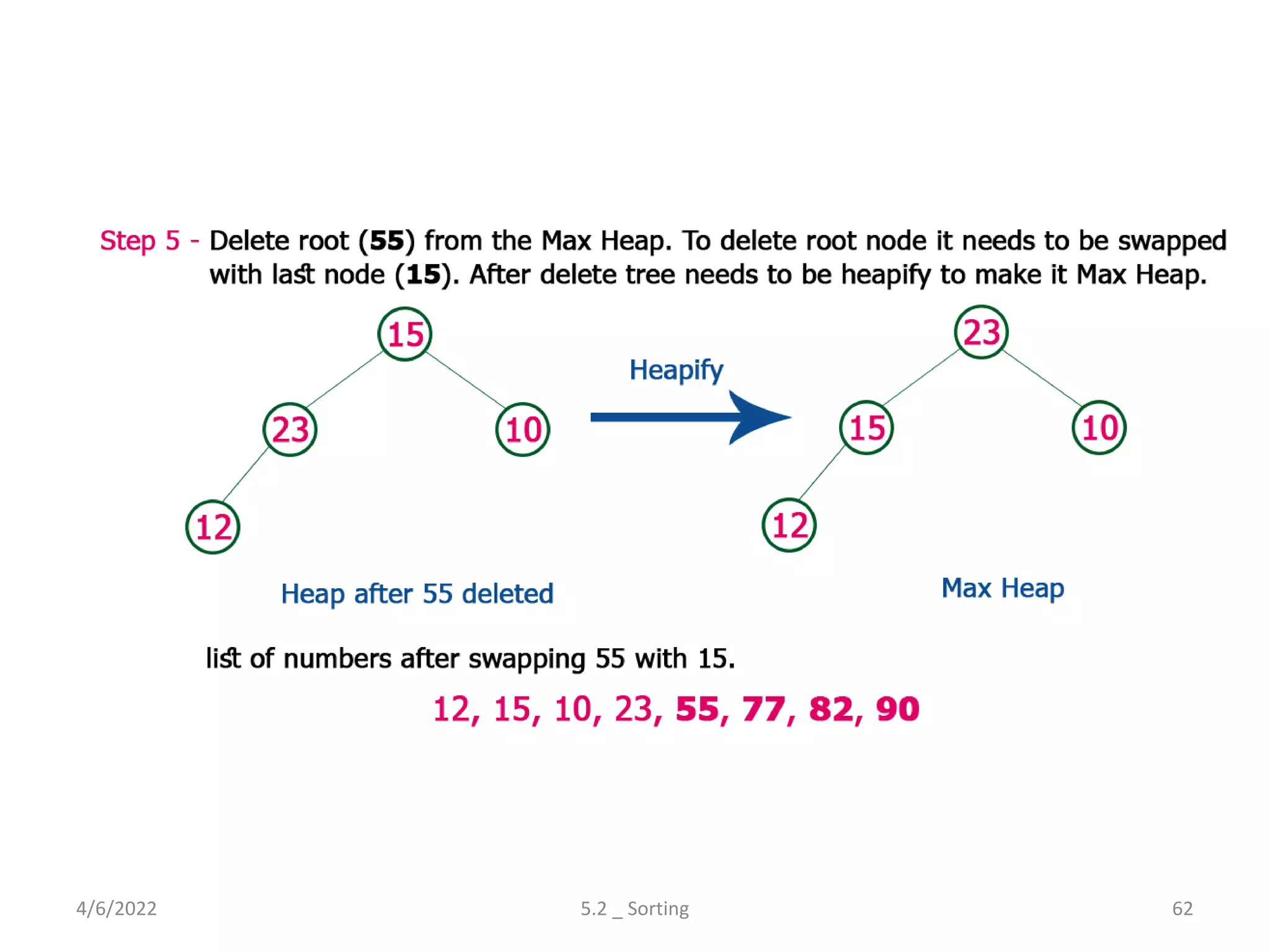
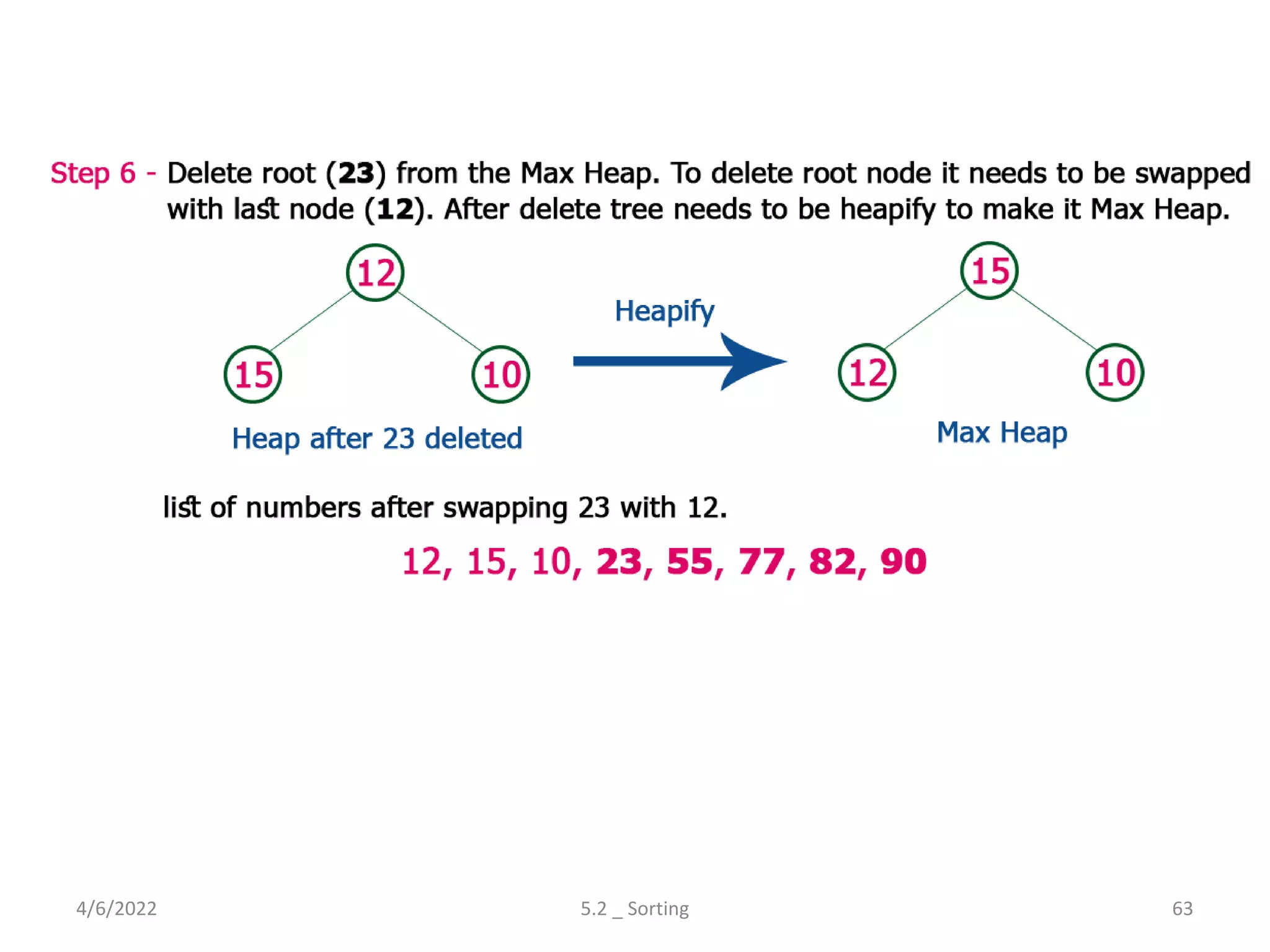
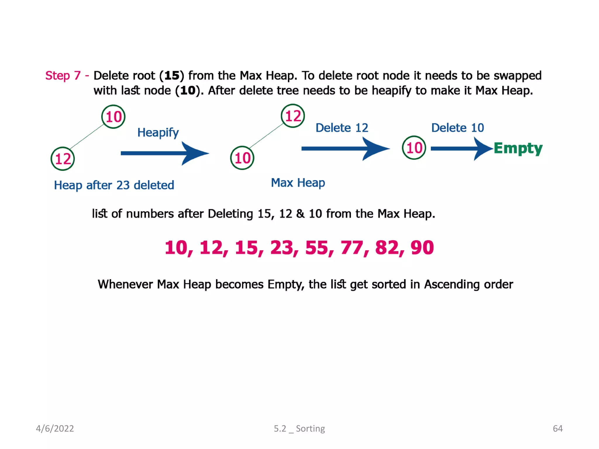
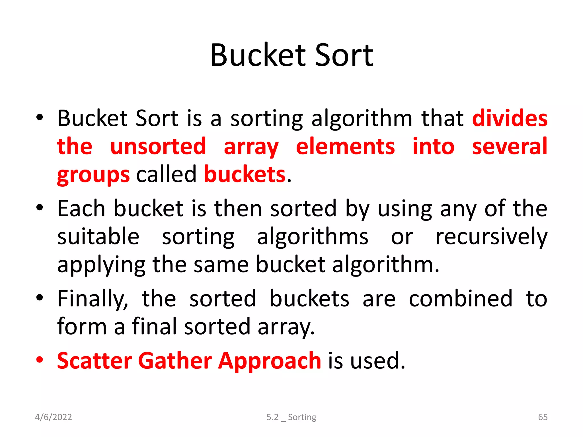
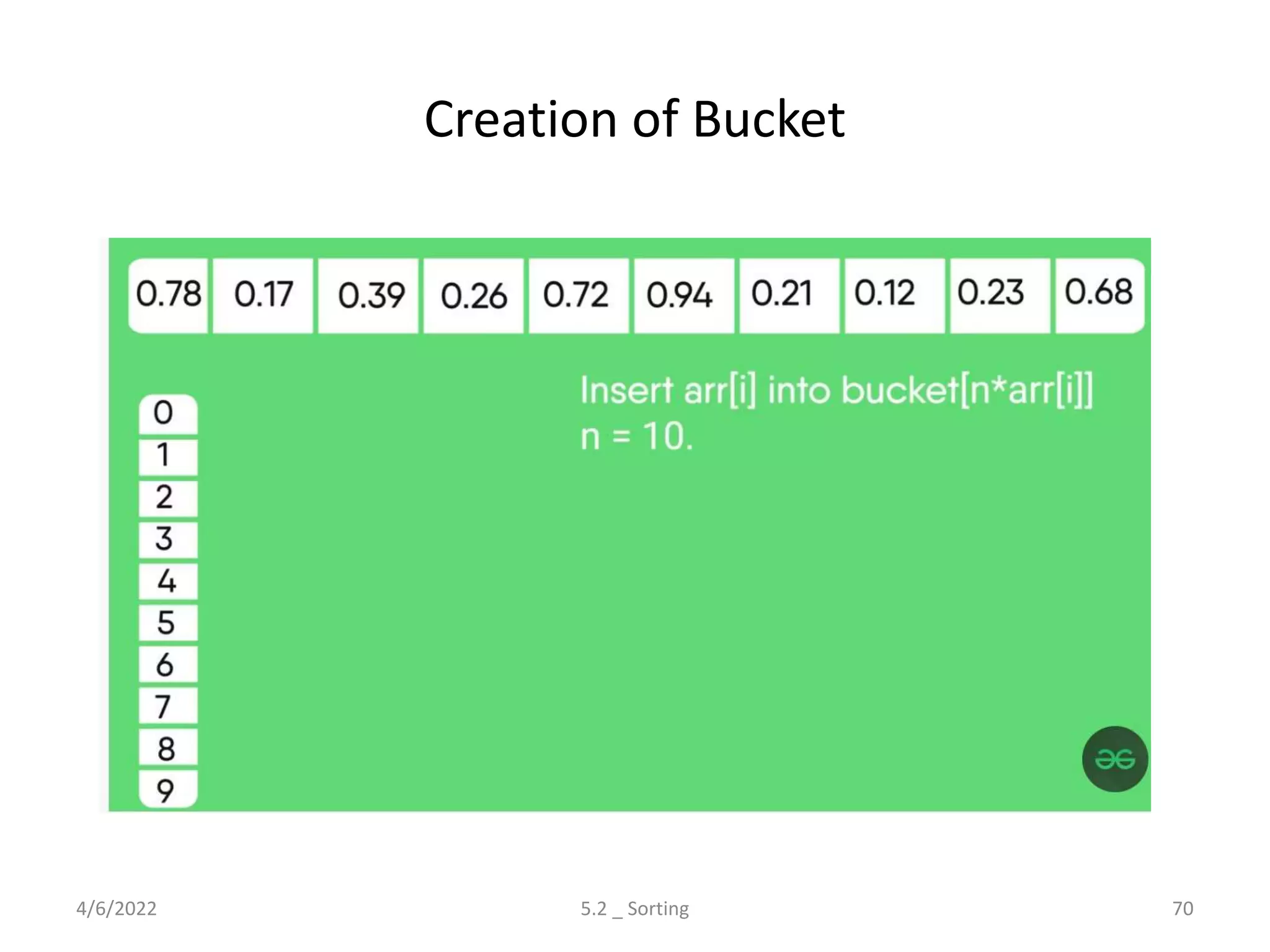
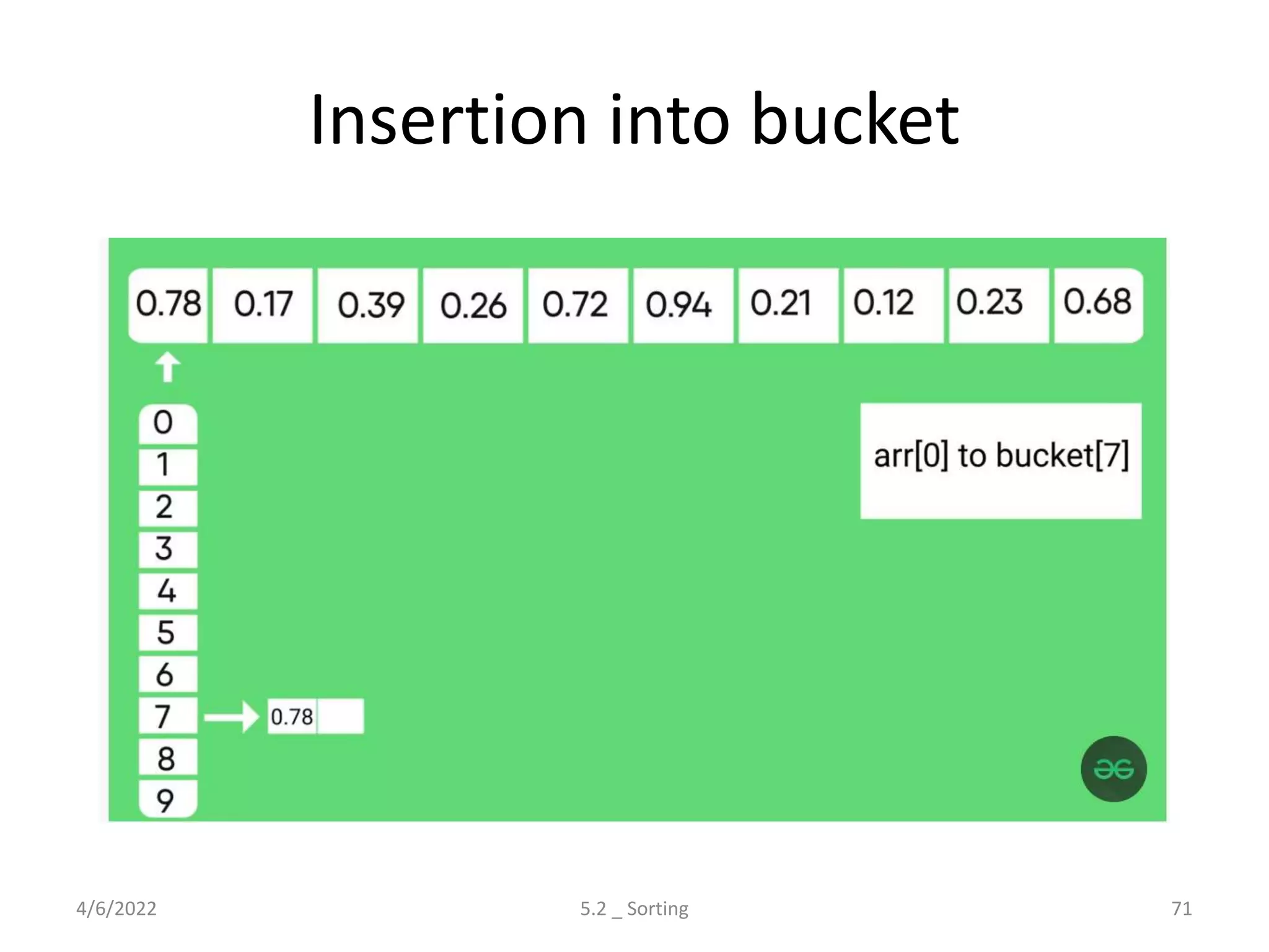
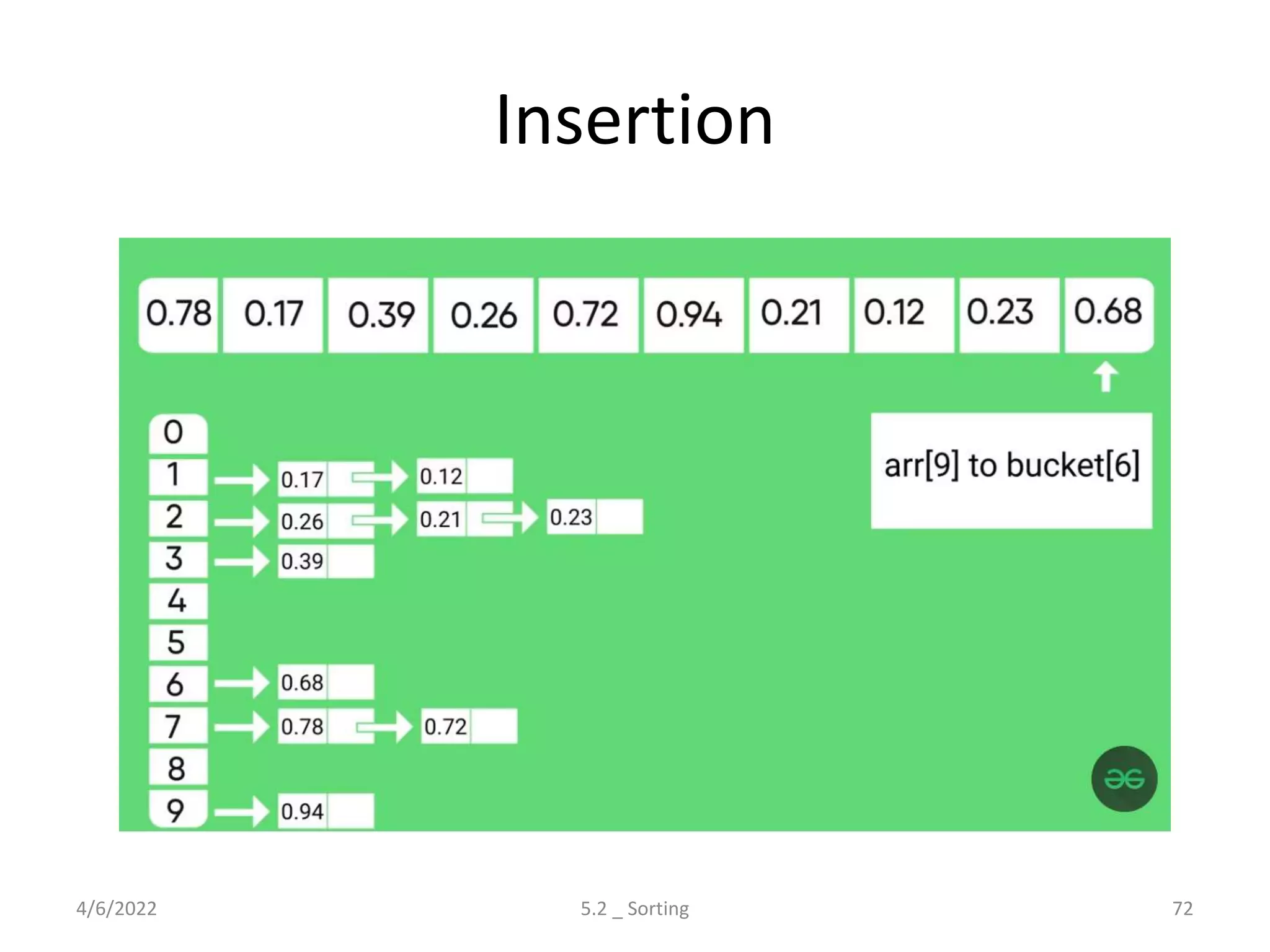
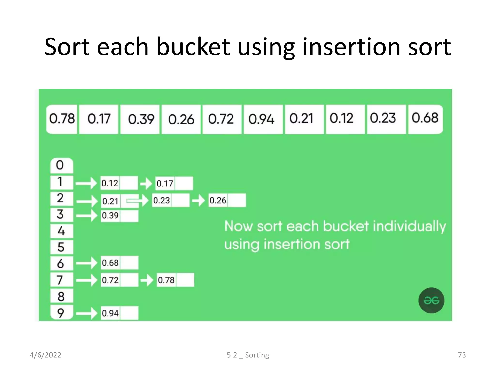
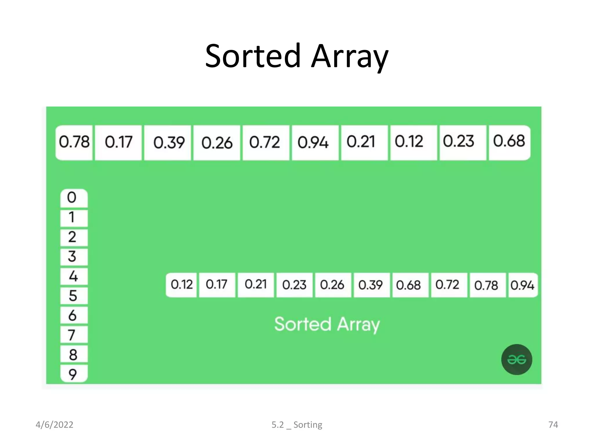
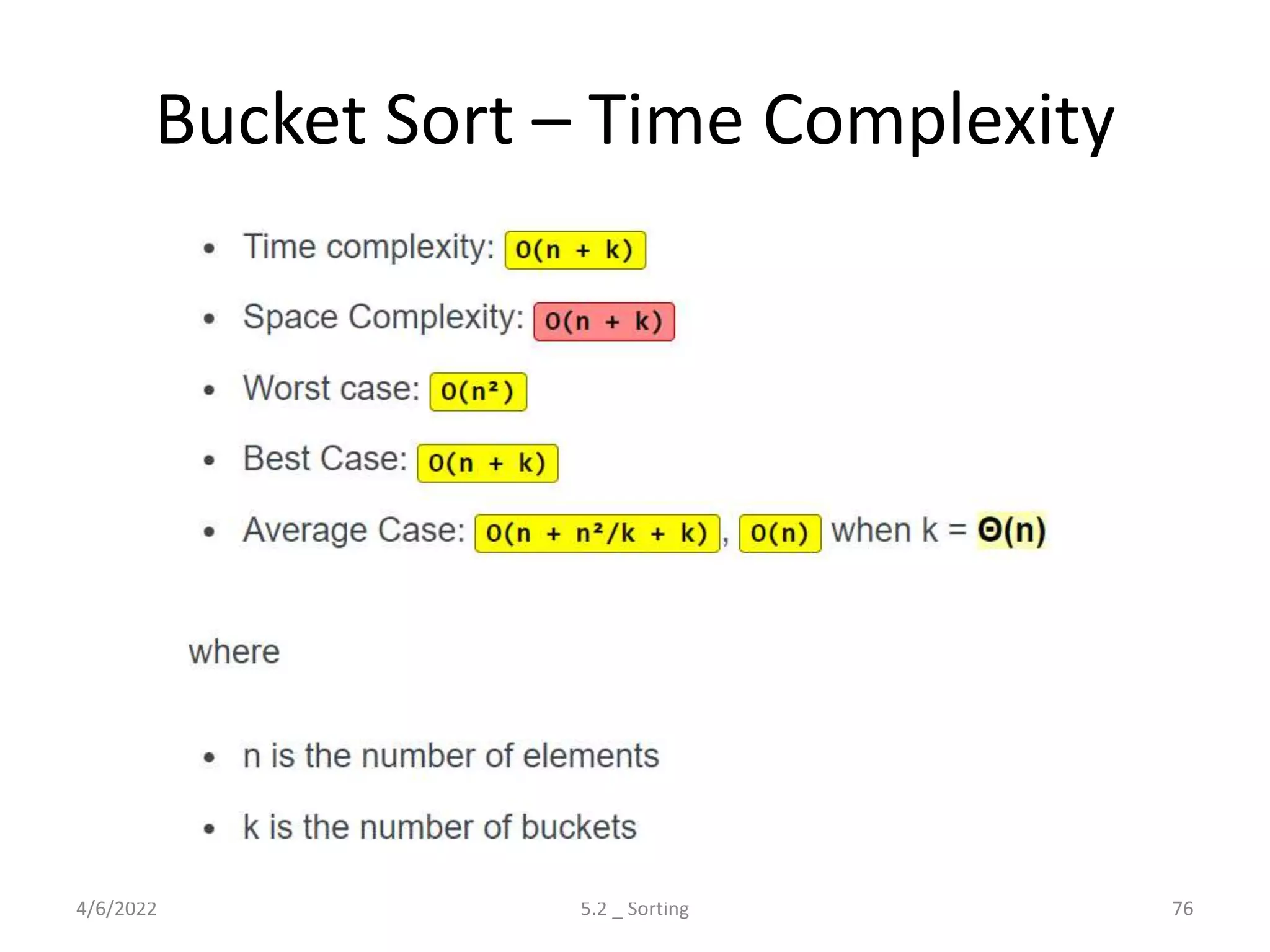
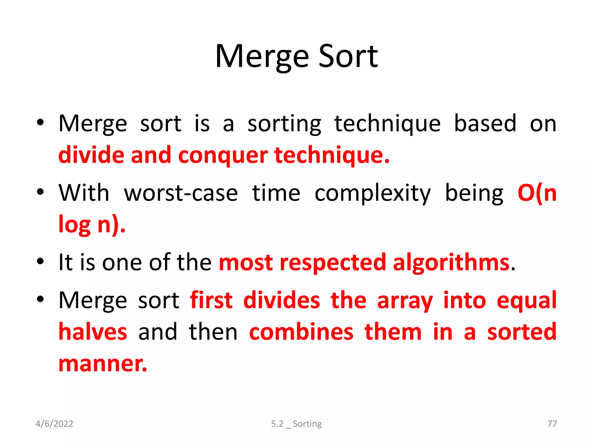
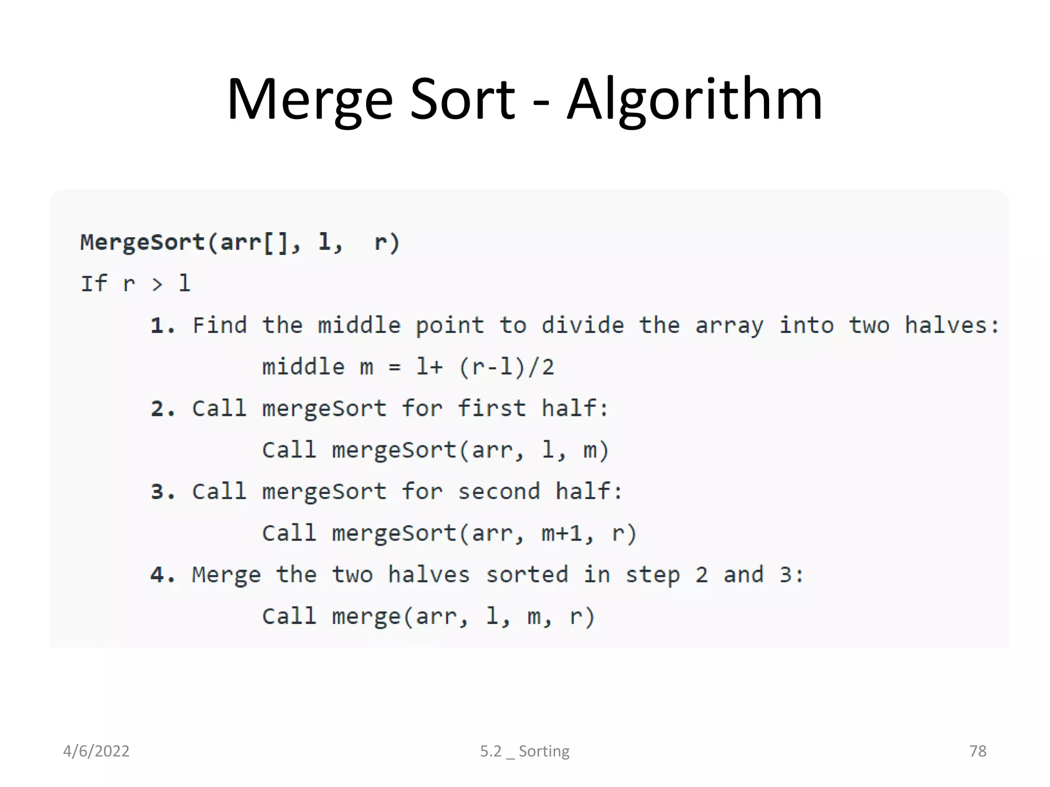
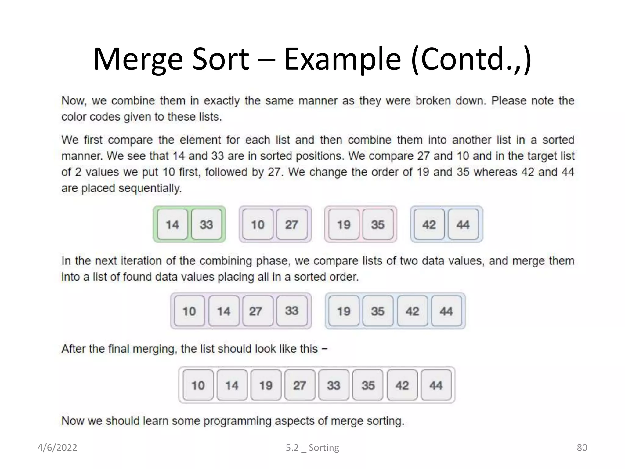
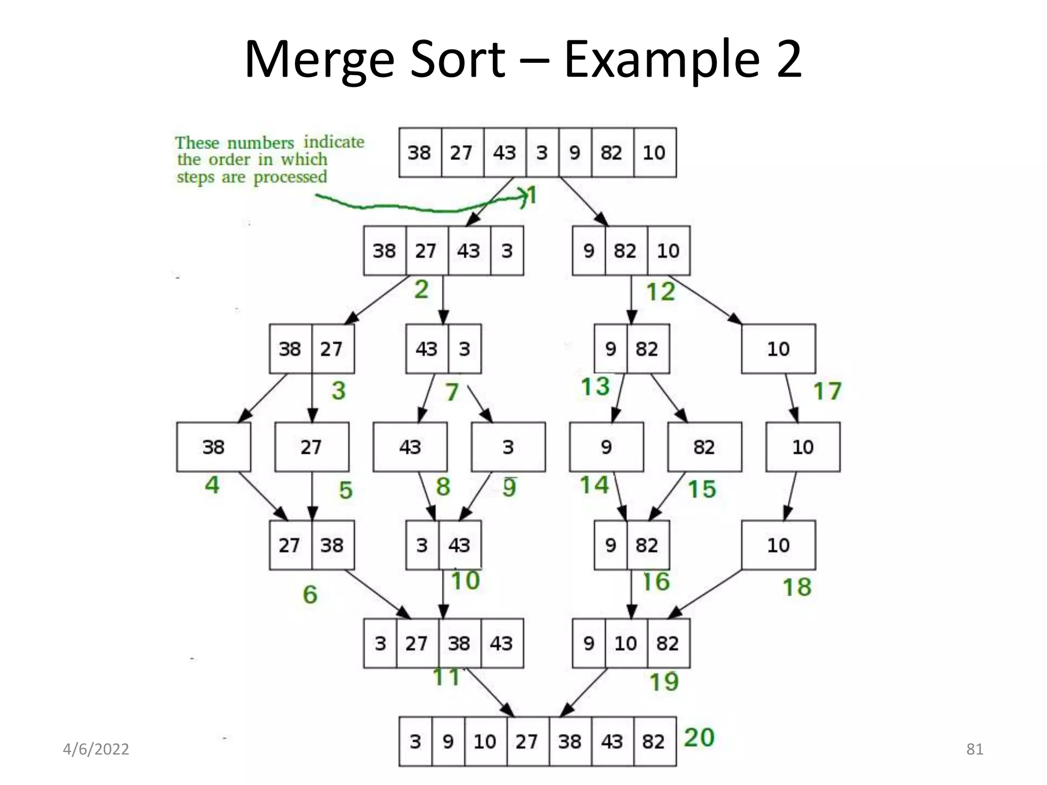
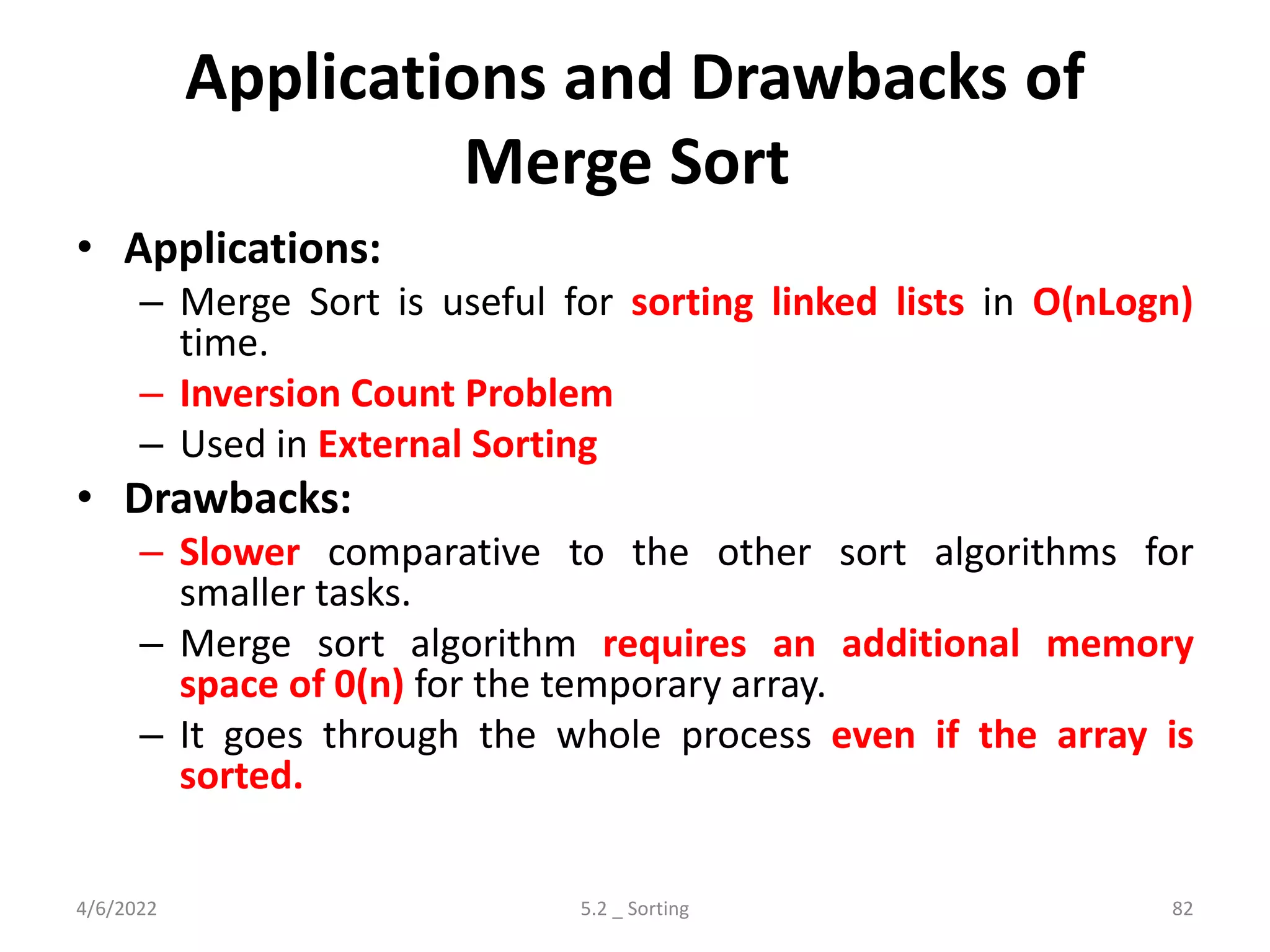
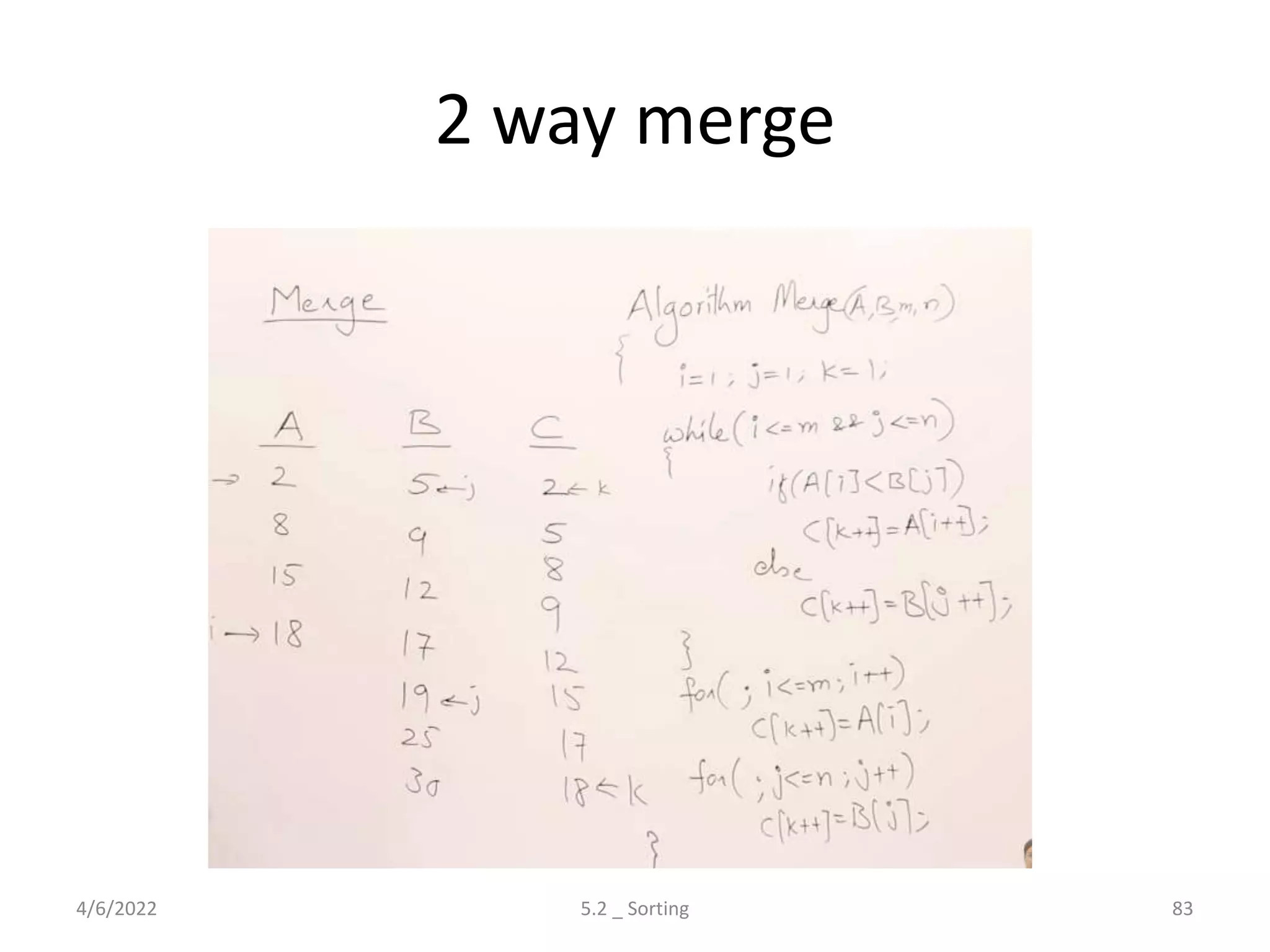
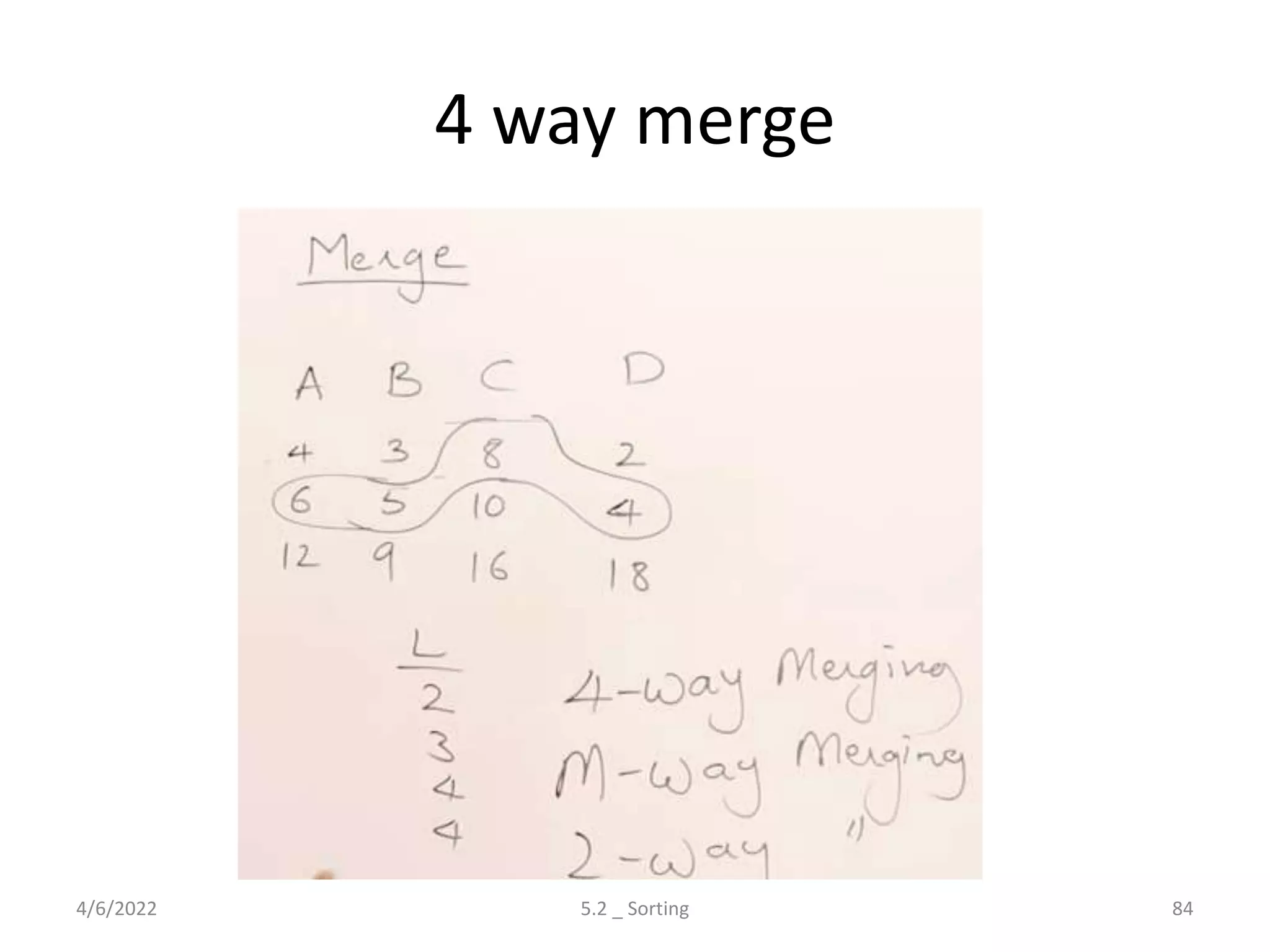
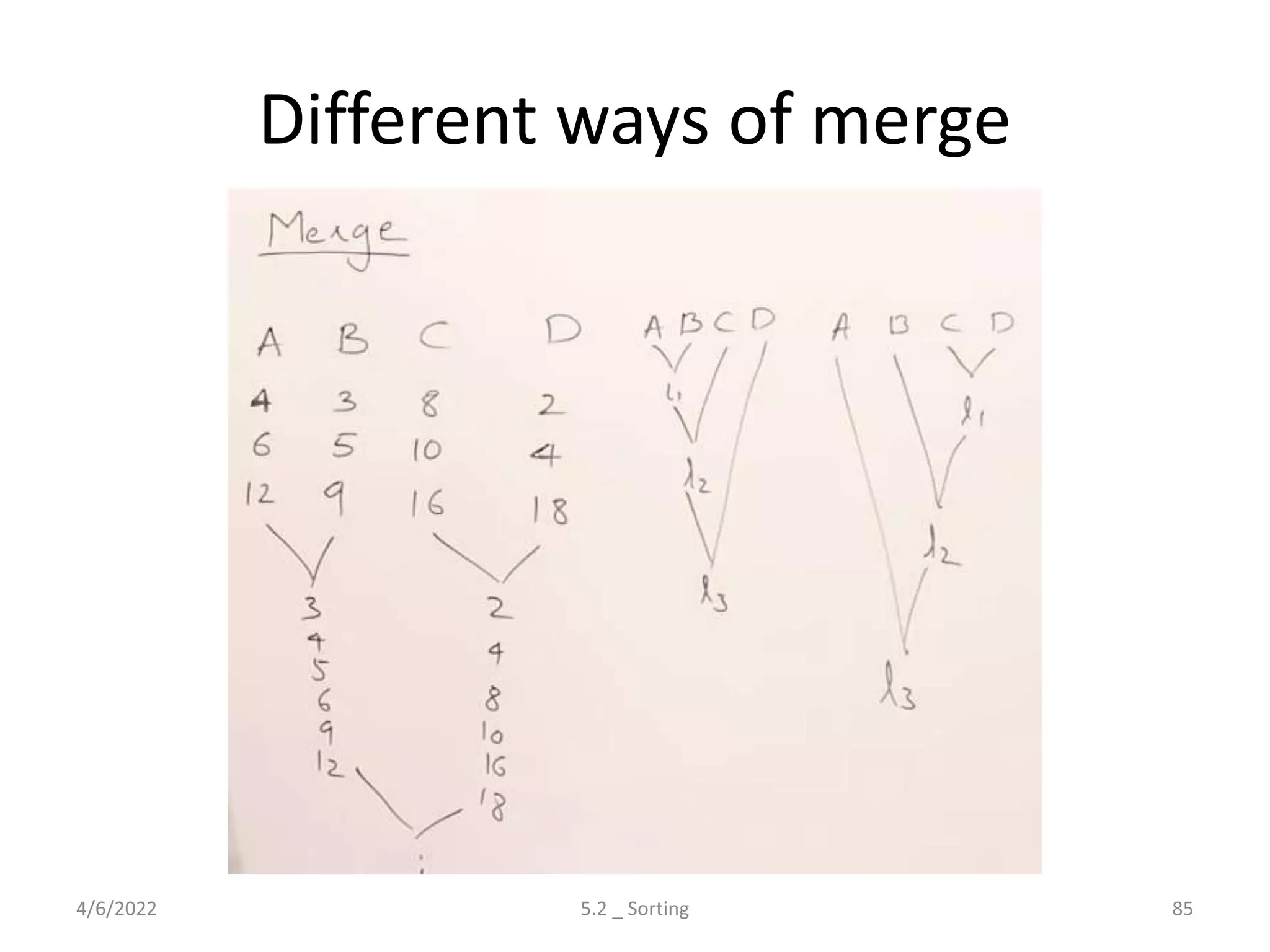
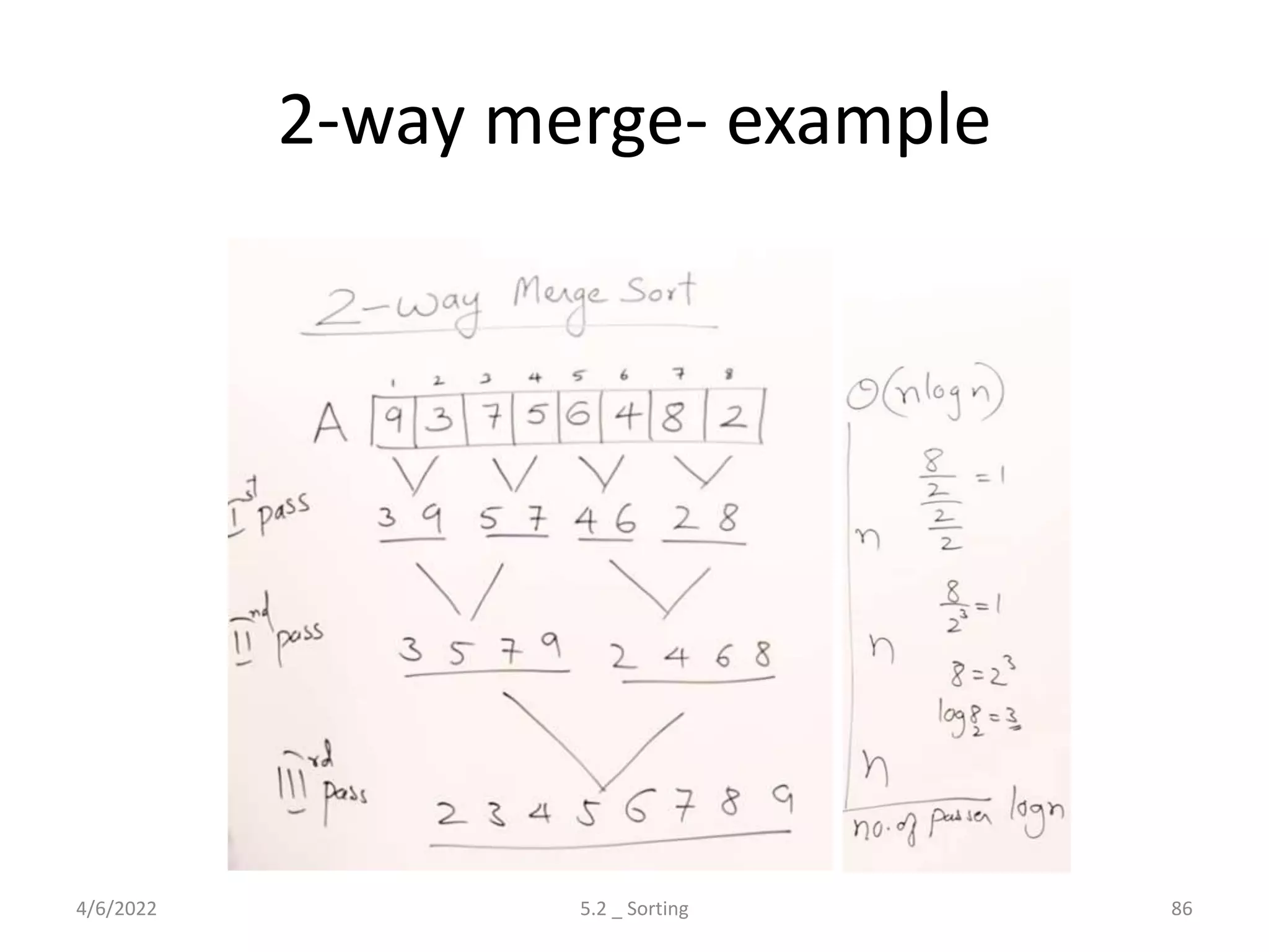
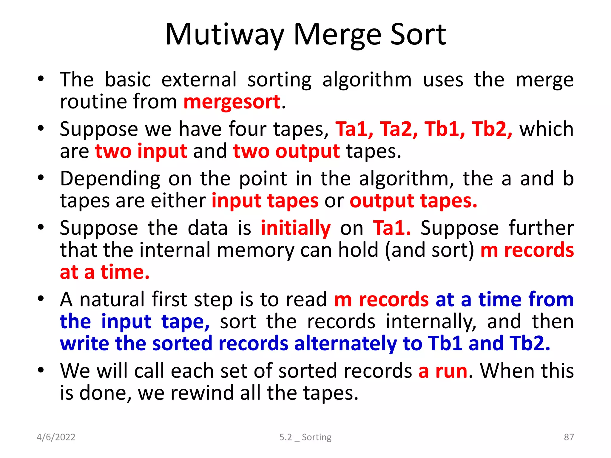
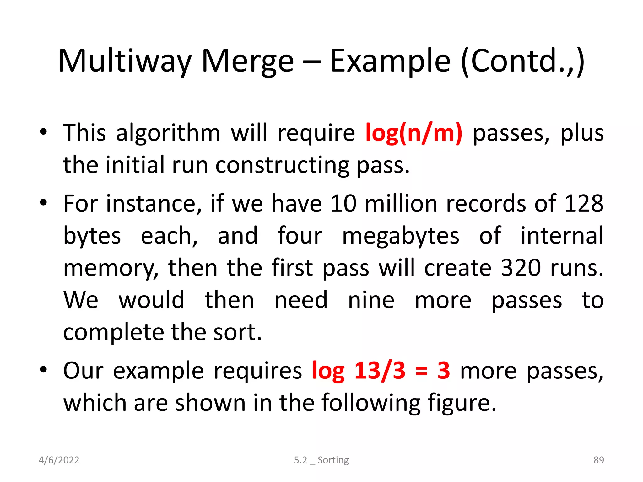
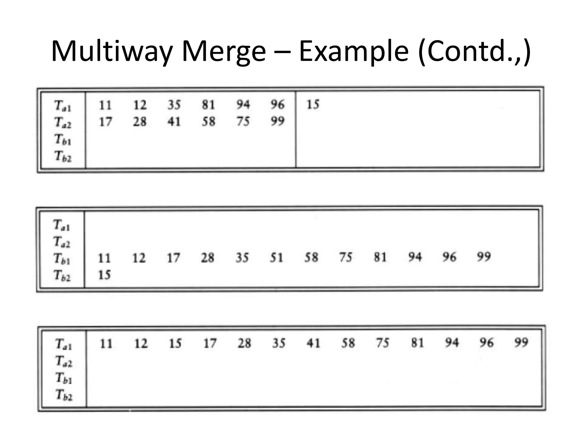
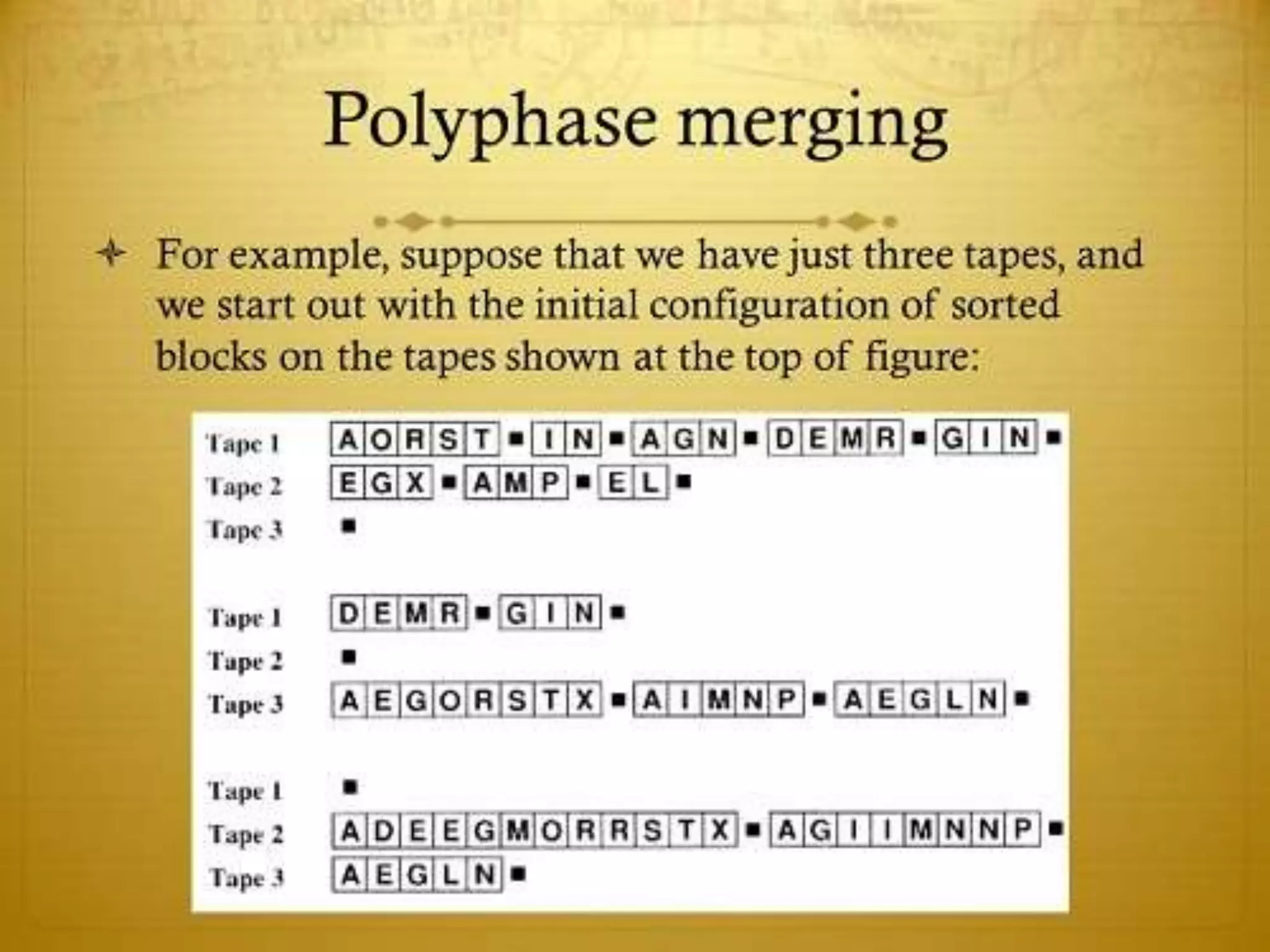
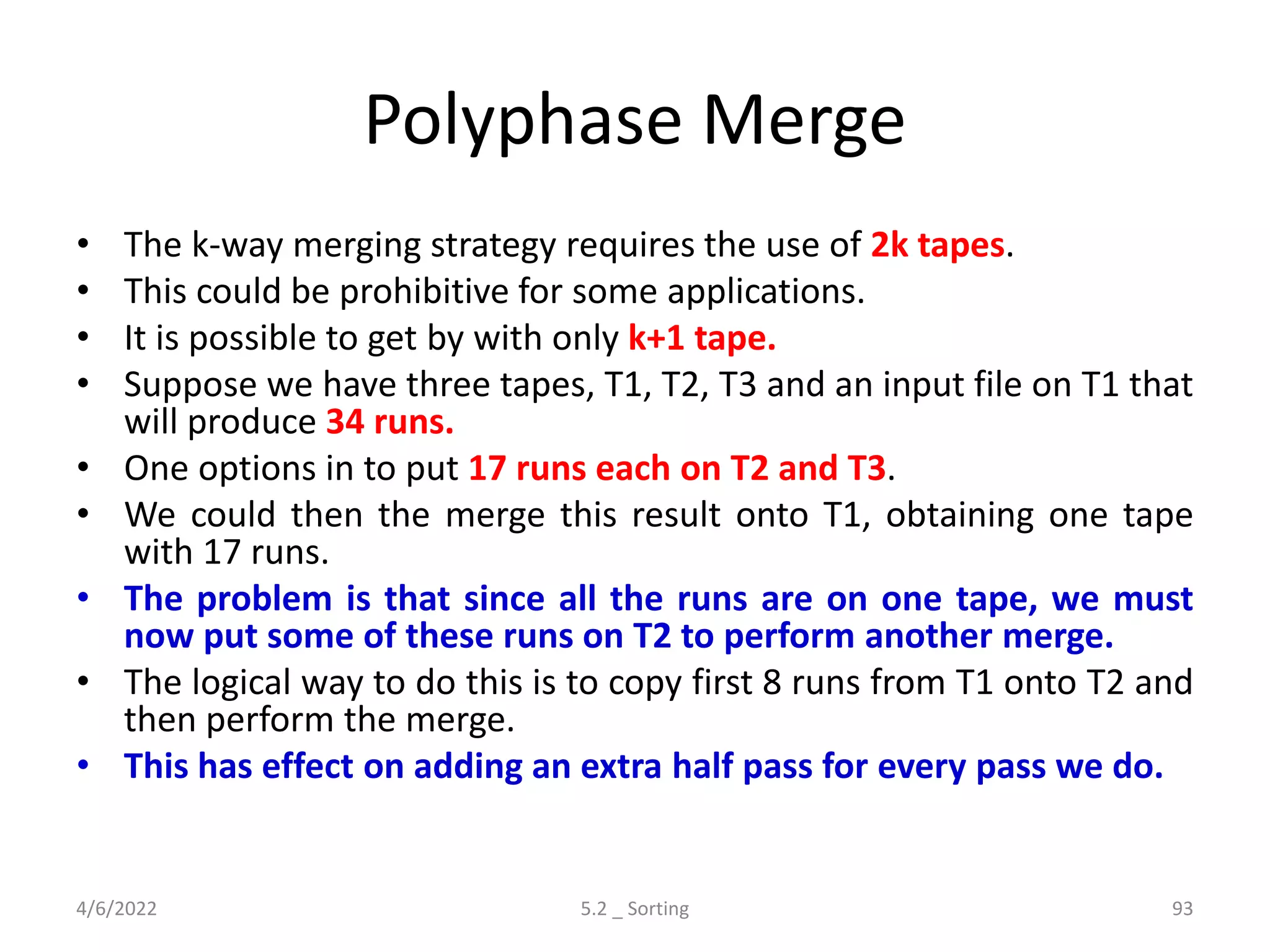
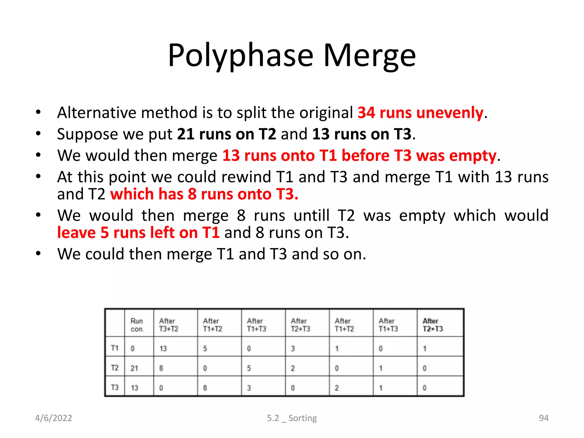
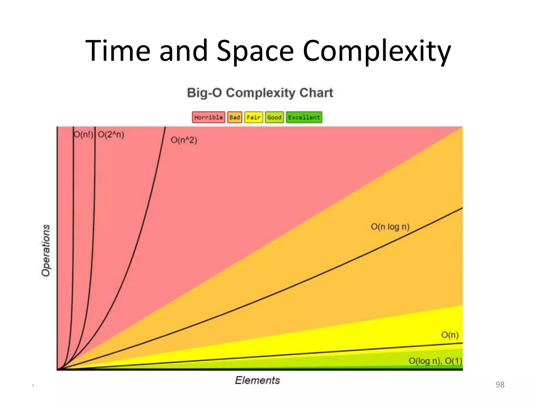
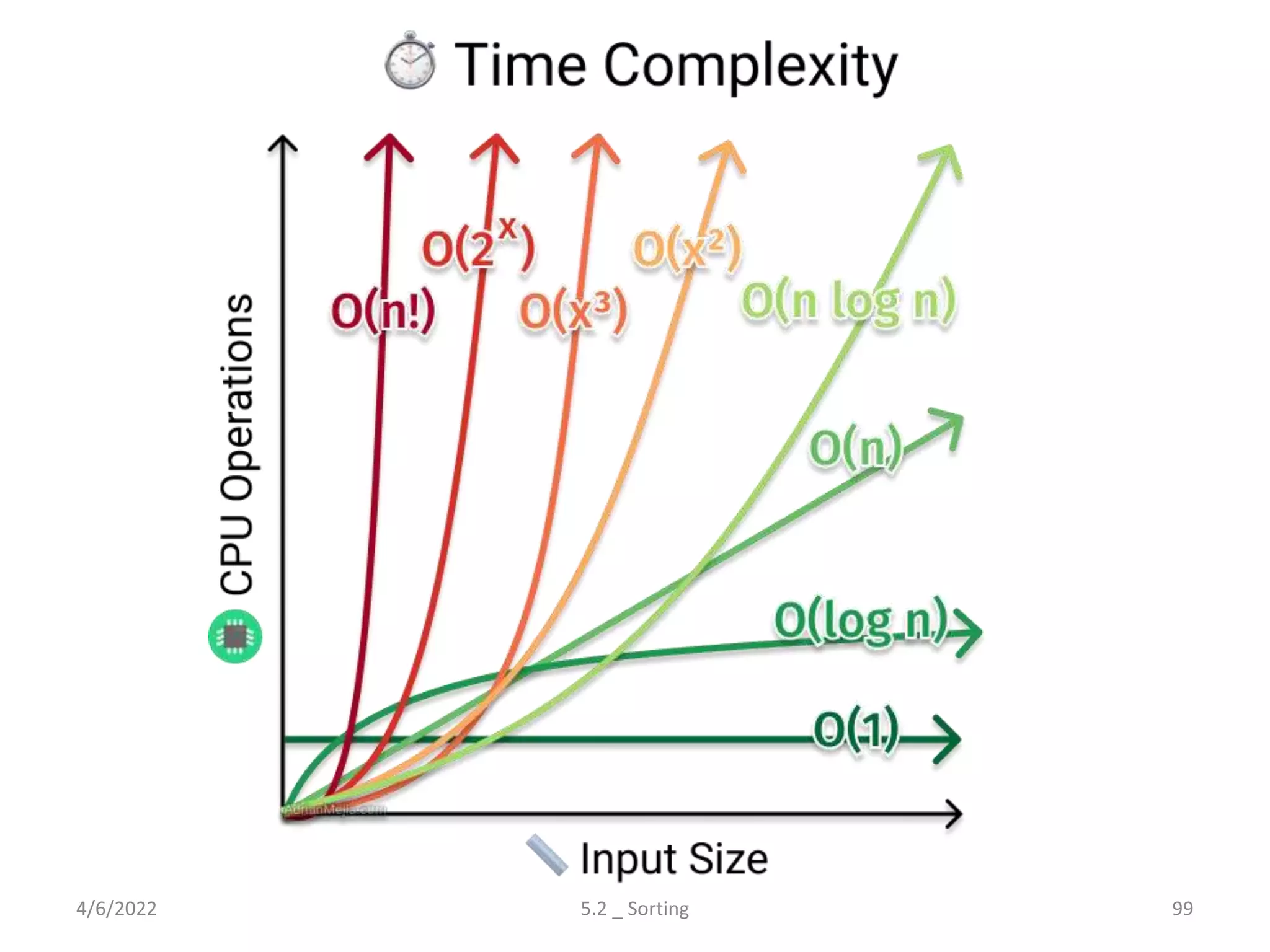
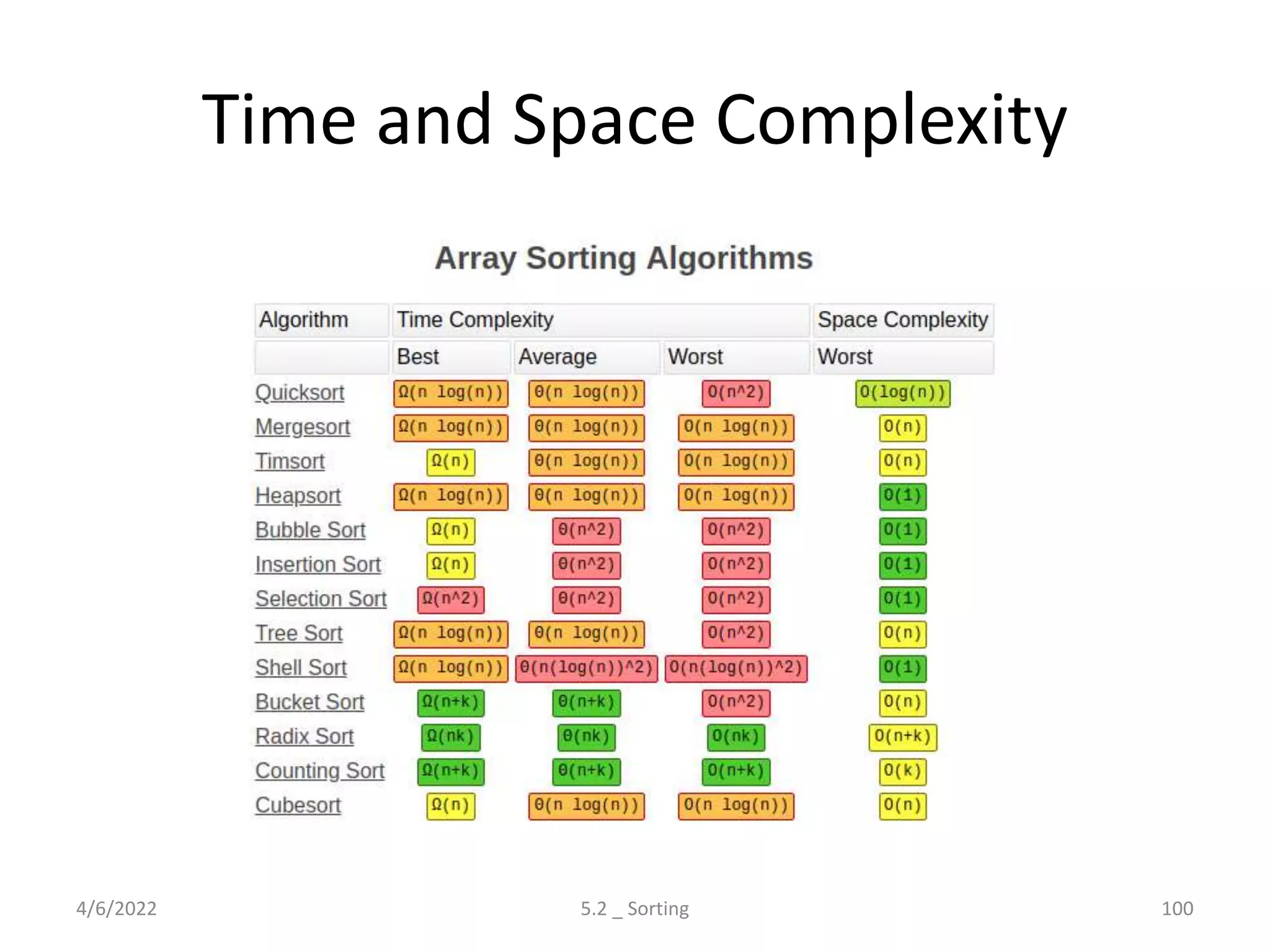
Explores various sorting techniques, including internal and external sorting. Key algorithms discussed are Insertion, Selection, Bubble, Shell, Quick, Heap, and Merge Sort.
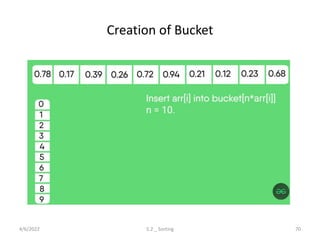
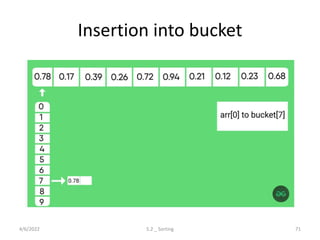
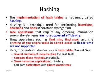
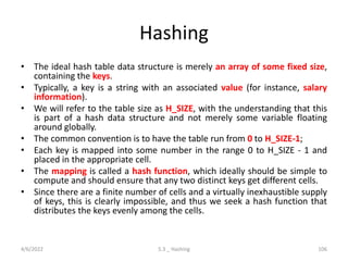
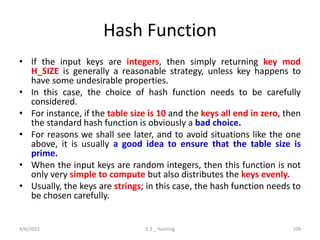
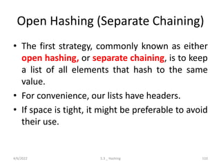
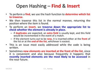
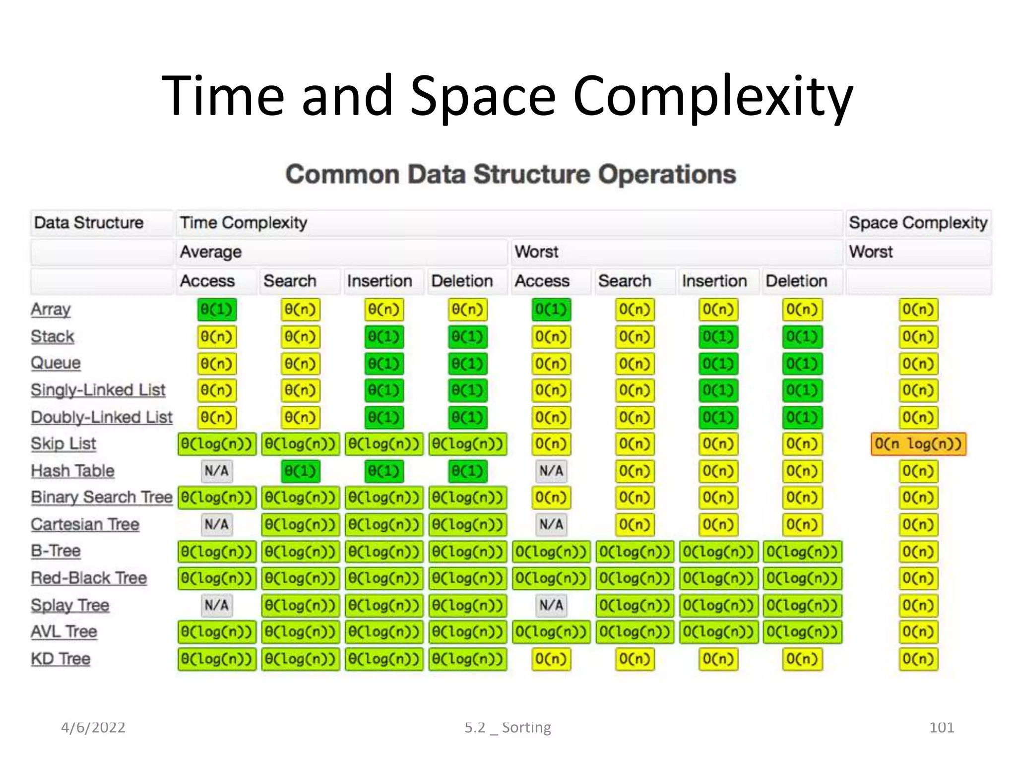
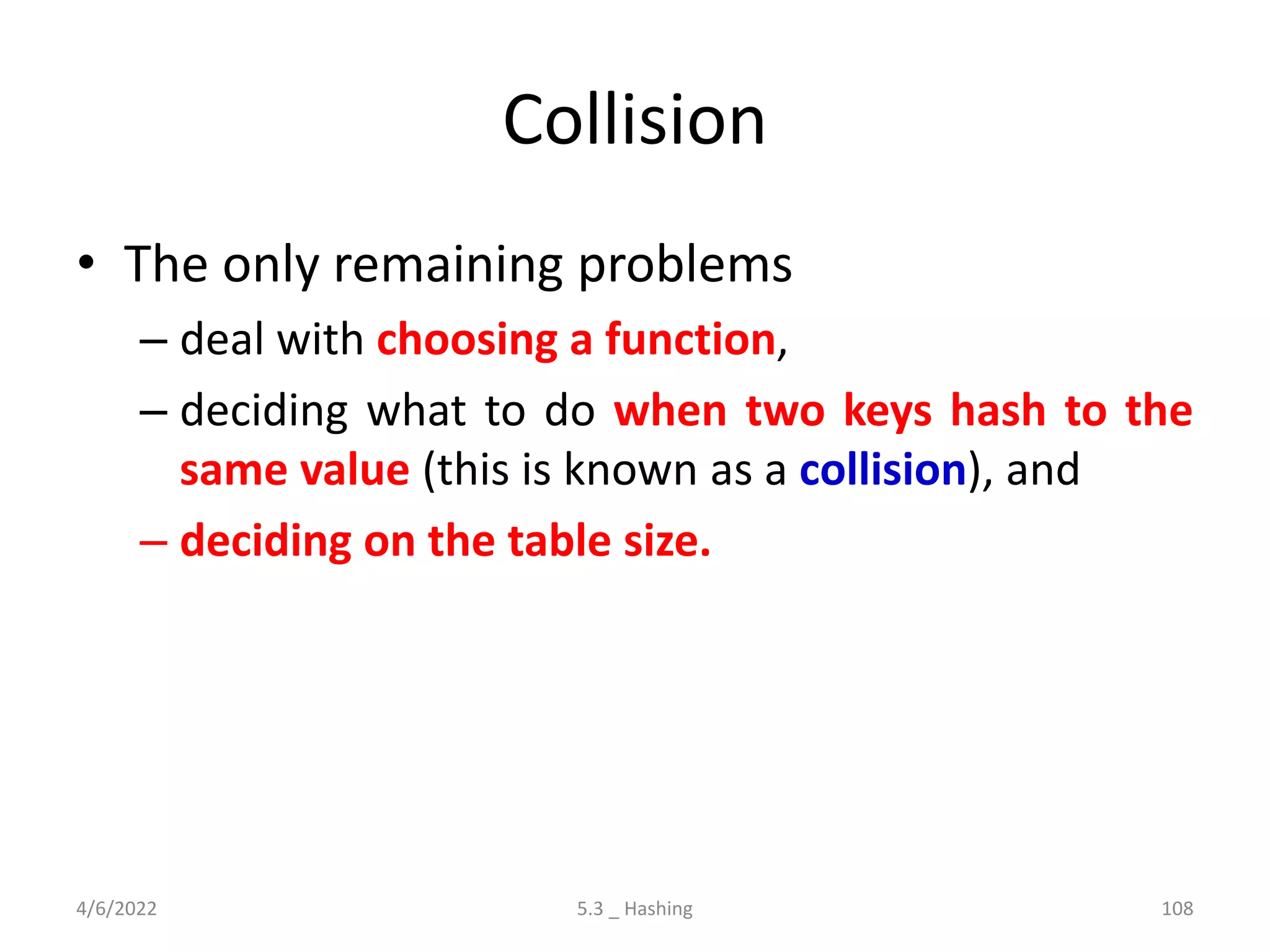
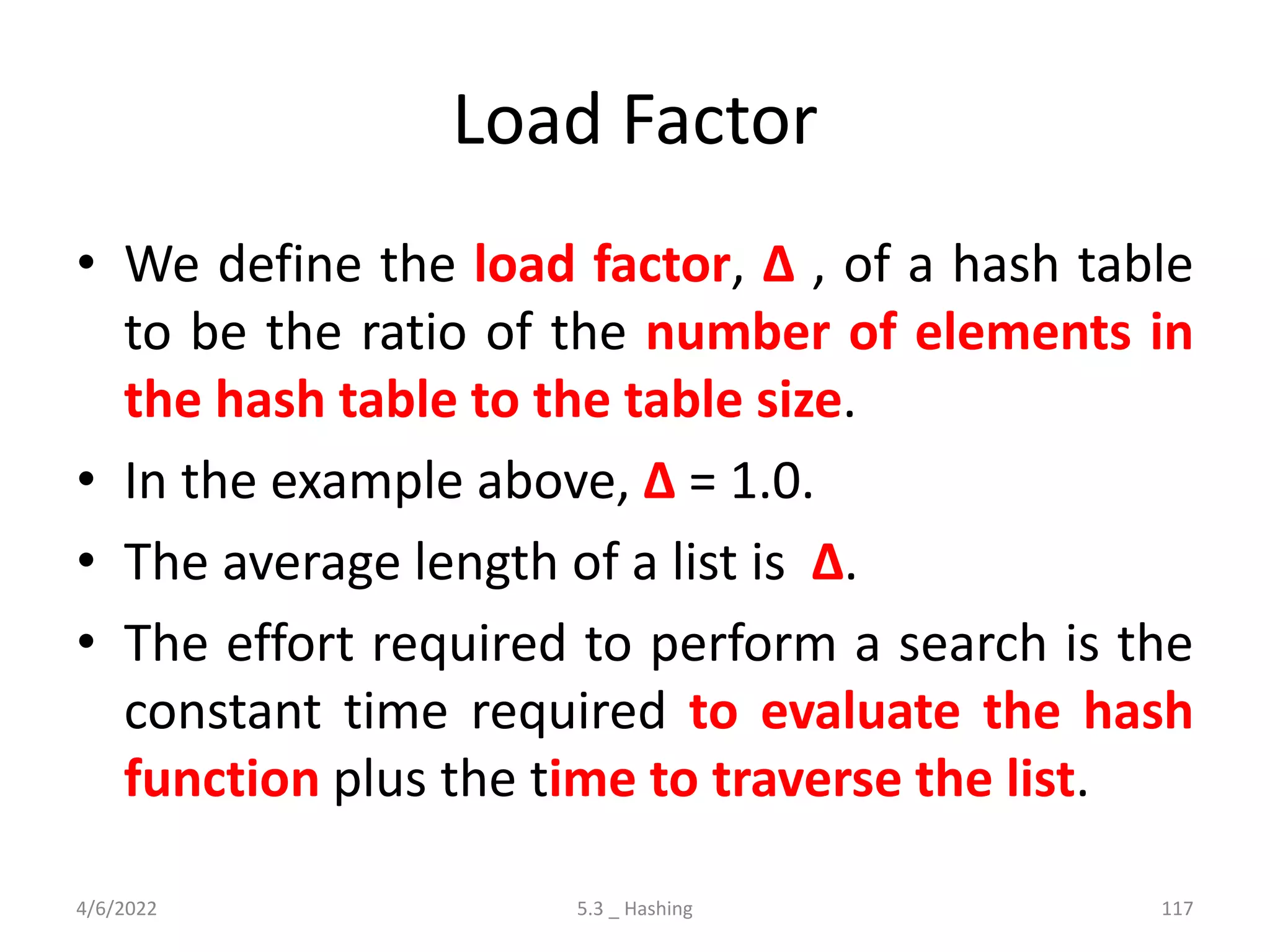
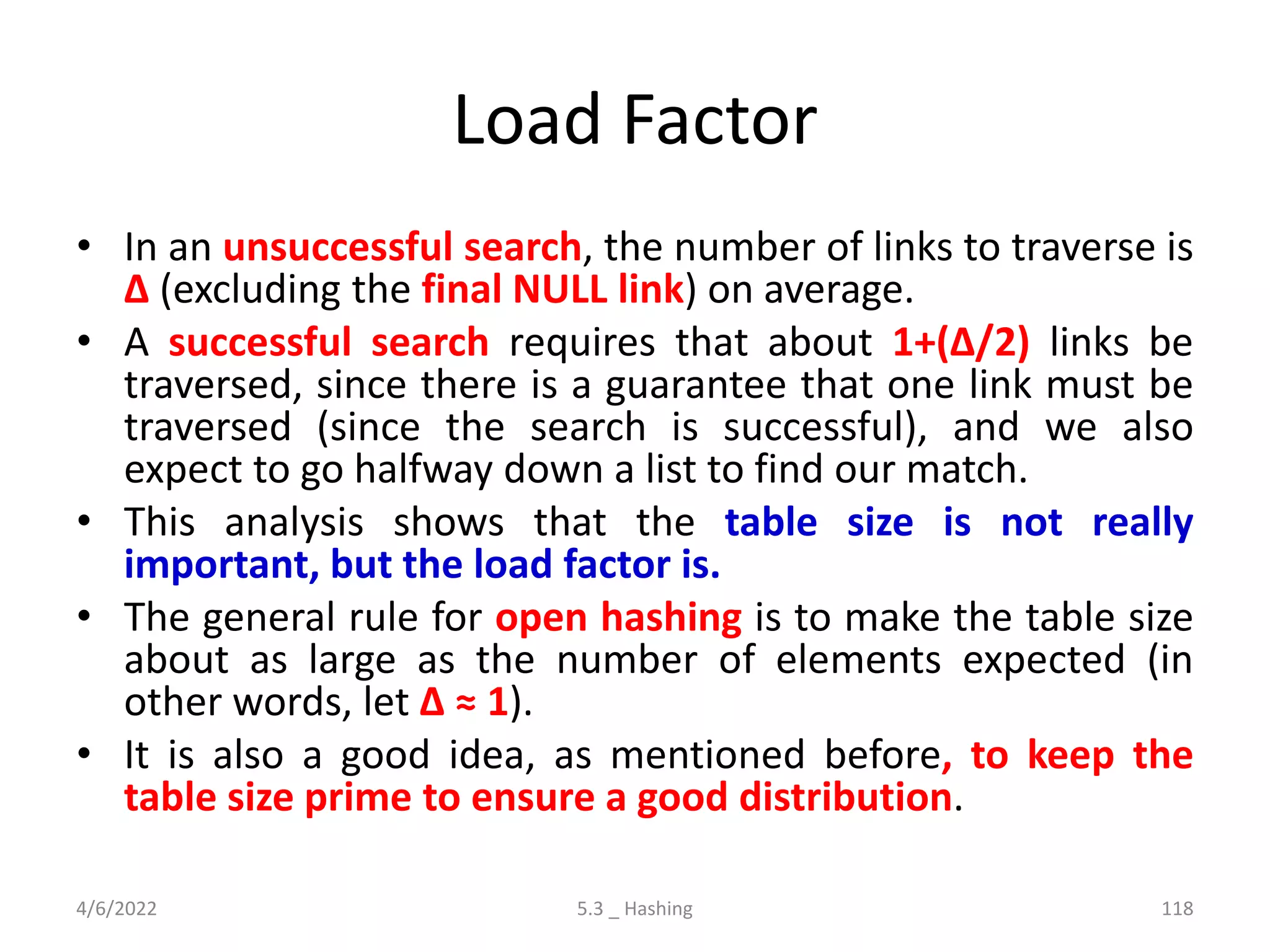
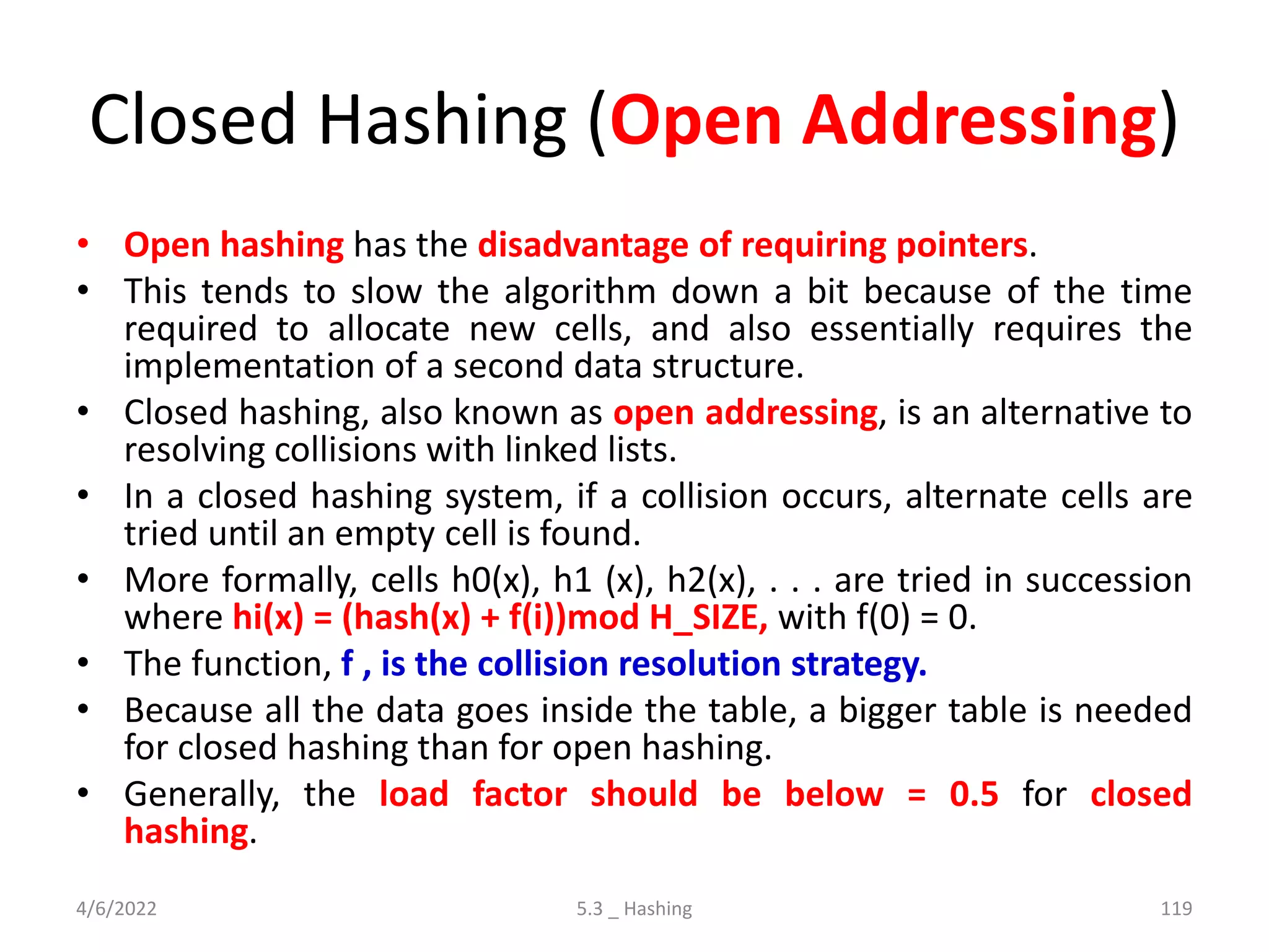
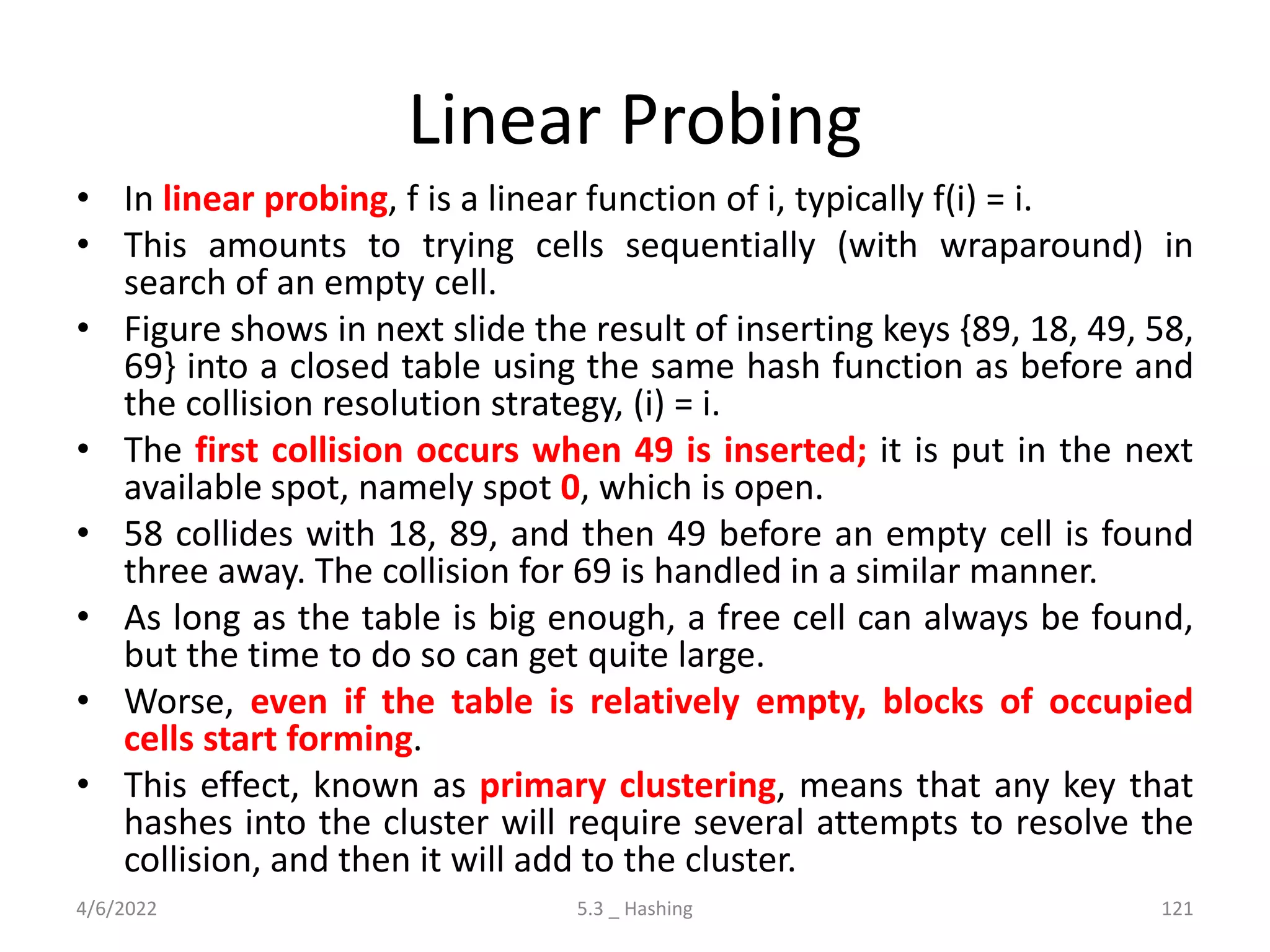
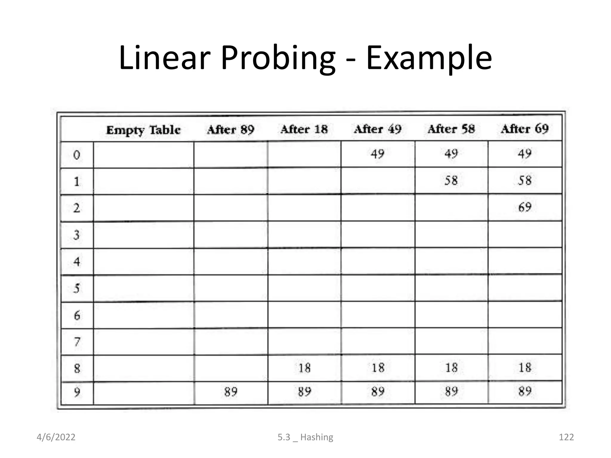
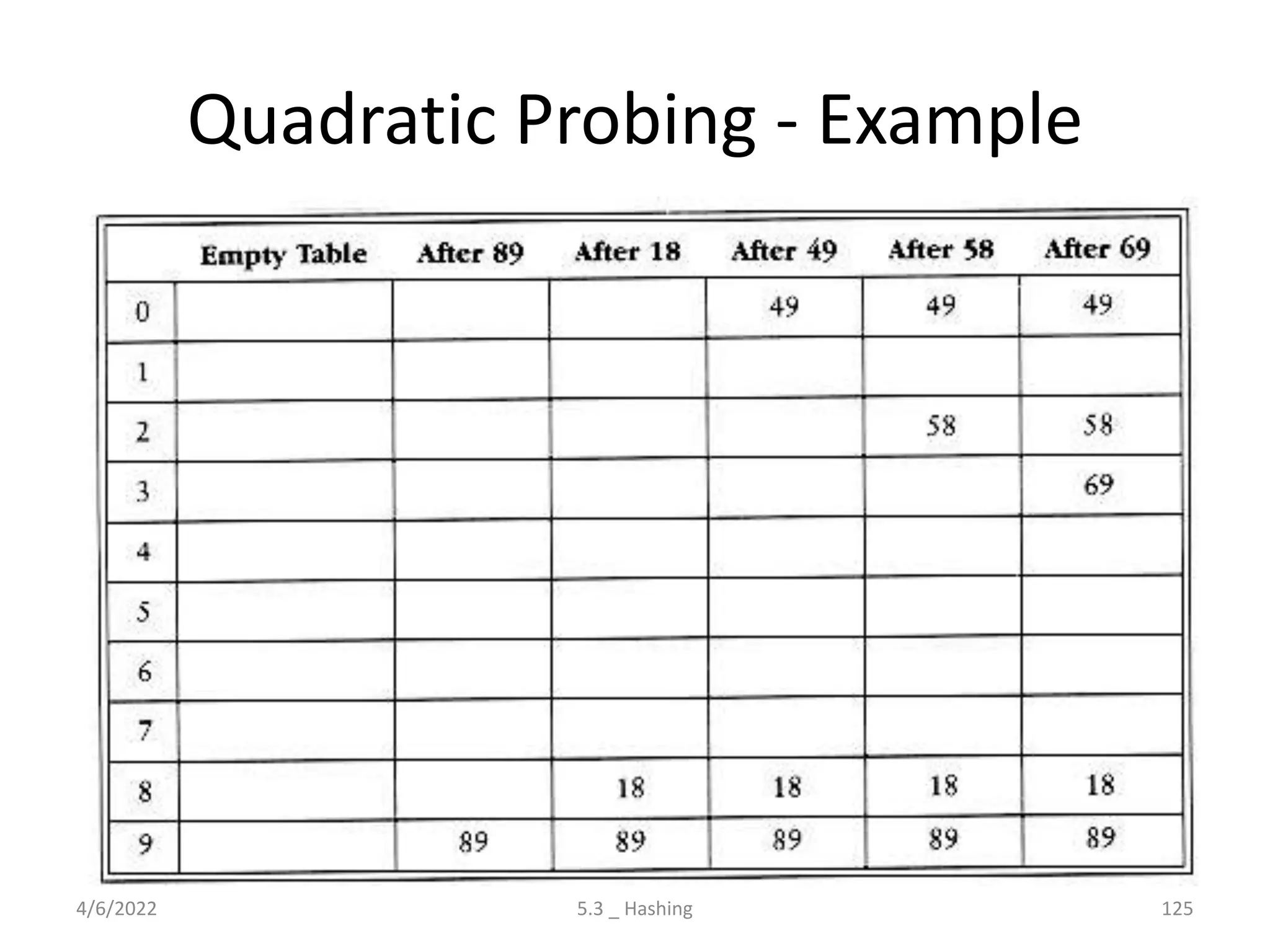
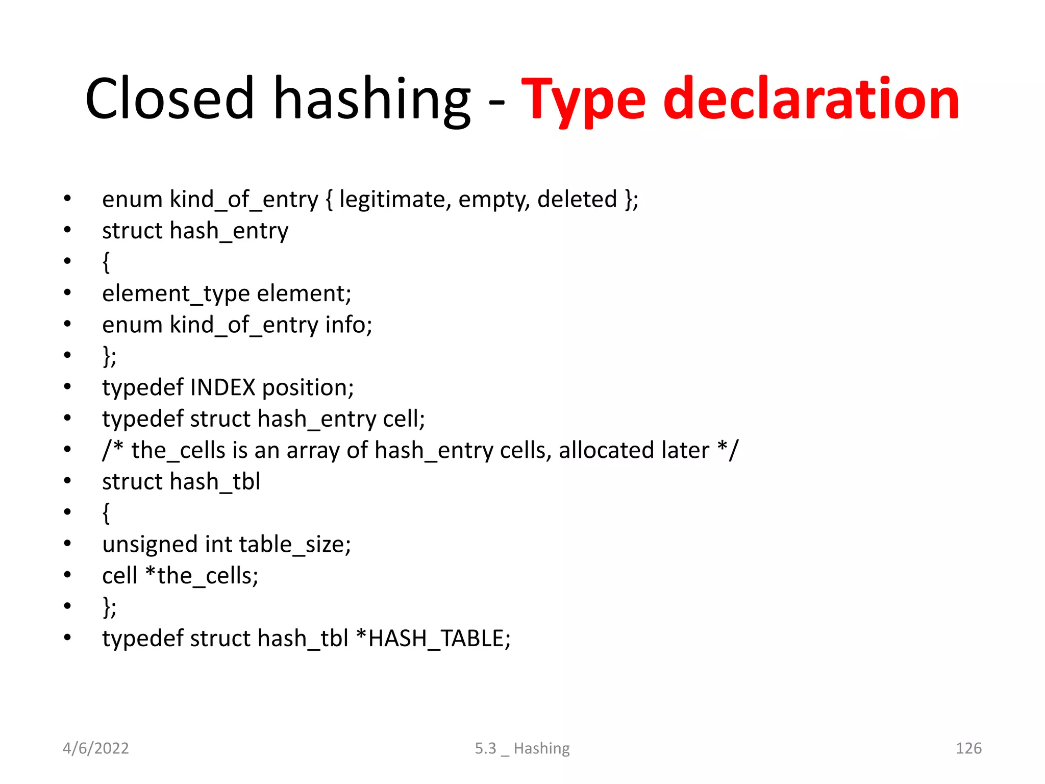
Introduces hashing, its applications, collision resolution strategies, including open and closed hashing, and discusses rehashing and extendible hashing.


![Data Structures - Lecture 9 [Stack & Queue using Linked List]](https://cdn.slidesharecdn.com/ss_thumbnails/lecture-9stackqueueusinglinkedlist-150219032411-conversion-gate02-thumbnail.jpg?width=600ounds&width=560&fit=bounds)


![[PPT] _ Unit 5 _ Evolve.pptx](https://cdn.slidesharecdn.com/ss_thumbnails/pptunit5evolve-220707120639-5c6df843-thumbnail.jpg?width=600ounds&width=560&fit=bounds)
![[PPT] _ Unit 4 _ Engage.pptx](https://cdn.slidesharecdn.com/ss_thumbnails/pptunit4engage-220707115545-9dce3530-thumbnail.jpg?width=600ounds&width=560&fit=bounds)
![[PPT] _ Unit 3 _ Experiment.pptx](https://cdn.slidesharecdn.com/ss_thumbnails/pptunit3experiment-220707114954-1996fe08-thumbnail.jpg?width=600ounds&width=560&fit=bounds)


![[PPT] _ UNIT 1 _ COMPLETE.pptx](https://cdn.slidesharecdn.com/ss_thumbnails/pptunit1complete-220516121012-45cab1a3-thumbnail.jpg?width=600ounds&width=560&fit=bounds)


![[PPT] _ Unit 2 _ 9.0 _ Domain Specific IoT _Home Automation.pdf](https://cdn.slidesharecdn.com/ss_thumbnails/pptunit29-220516115946-098632b6-thumbnail.jpg?width=600ounds&width=560&fit=bounds)


