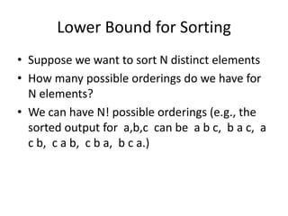
Downloaded 39 times

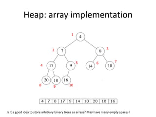
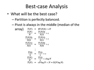
![Array implementation1632514The root node is A[1].The left child of A[j] is A[2j]The right child of A[j] is A[2j + 1]The parent of A[j] is A[j/2] (note: integer divide)25436Need to estimate the maximum size of the heap.](https://image.slidesharecdn.com/sorting2-110225223207-phpapp02/85/Sorting2-5-320.jpg)


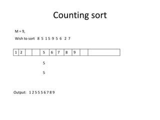
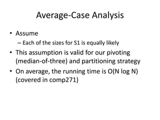
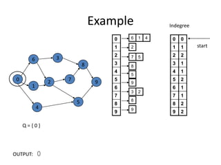
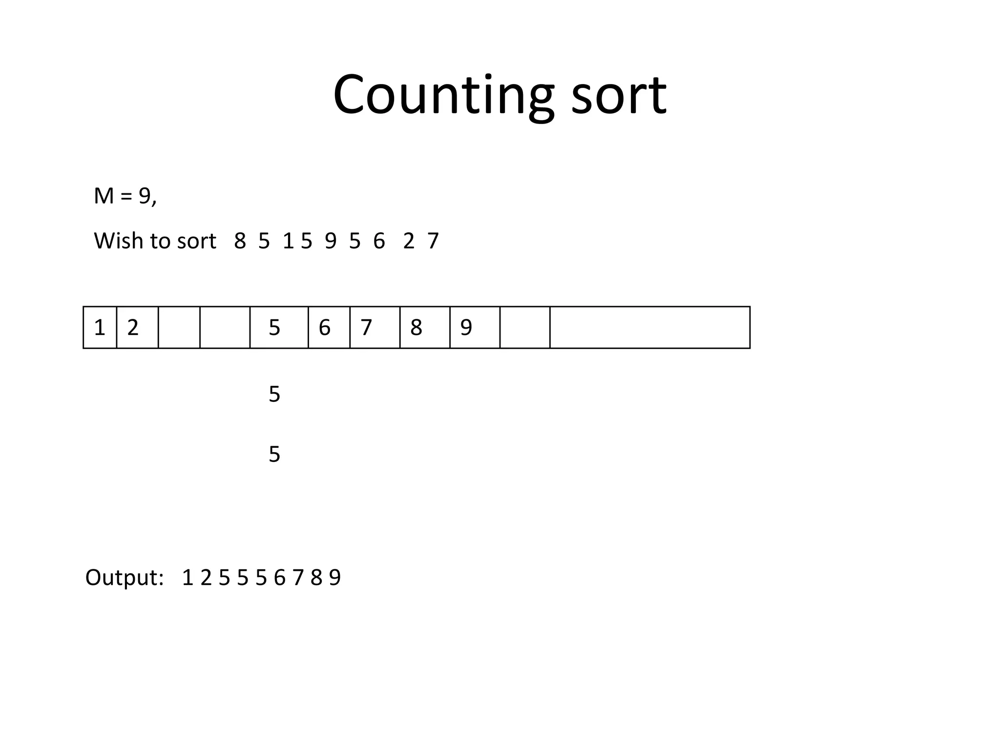
![Counting SortAssume N integers to be sorted, each is in the range 1 to M.Define an array B[1..M], initialize all to 0 O(M)Scan through the input list A[i], insert A[i] into B[A[i]] O(N)Scan B once, read out the nonzero integers O(M)Total time: O(M + N)if M is O(N), then total time is O(N)Can be bad if range is very big, e.g. M=O(N2)N=7, M = 9, Want to sort 8 1 9 5 2 6 3 5893612Output: 1 2 3 5 6 8 9](https://image.slidesharecdn.com/sorting2-110225223207-phpapp02/85/Sorting2-22-320.jpg)
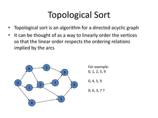
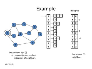
![Counting sortWhat if we have duplicates?B is an array of pointers.Each position in the array has 2 pointers: head and tail. Tail points to the end of a linked list, and head points to the beginning.A[j] is inserted at the end of the list B[A[j]]Again, Array B is sequentially traversed and each nonempty list is printed out.Time: O(M + N)](https://image.slidesharecdn.com/sorting2-110225223207-phpapp02/85/Sorting2-23-320.jpg)


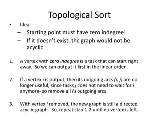
![// base 10// FIFO// d times of counting sort// scan A[i], put into correct slot// re-order back to original array](https://image.slidesharecdn.com/sorting2-110225223207-phpapp02/85/Sorting2-31-320.jpg)


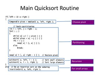
![Pseudocode Input: an array A[p, r]Quicksort (A, p, r) { if (p < r) { q = Partition (A, p, r) //q is the position of the pivot elementQuicksort (A, p, q-1)Quicksort (A, q+1, r) }}](https://image.slidesharecdn.com/sorting2-110225223207-phpapp02/85/Sorting2-38-320.jpg)
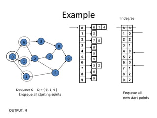
![Partitioning Strategy196jiWant to partition an array A[left .. right]First, get the pivot element out of the way by swapping it with the last element. (Swap pivot and A[right])Let i start at the first element and j start at the next-to-last element (i = left, j = right – 1)swap656431219564312pivot](https://image.slidesharecdn.com/sorting2-110225223207-phpapp02/85/Sorting2-40-320.jpg)
![Partitioning Strategy191966jjiiWant to haveA[p] <= pivot, for p < iA[p] >= pivot, for p > jWhen i < jMove i right, skipping over elements smaller than the pivotMove j left, skipping over elements greater than the pivotWhen both i and j have stoppedA[i] >= pivotA[j] <= pivot564312564312](https://image.slidesharecdn.com/sorting2-110225223207-phpapp02/85/Sorting2-41-320.jpg)
![Partitioning Strategy191966jjiiWhen i and j have stopped and i is to the left of jSwap A[i] and A[j]The large element is pushed to the right and the small element is pushed to the leftAfter swappingA[i] <= pivotA[j] >= pivotRepeat the process until i and j crossswap564312534612](https://image.slidesharecdn.com/sorting2-110225223207-phpapp02/85/Sorting2-42-320.jpg)
![Partitioning Strategy191919666jjjiiiWhen i and j have crossedSwap A[i] and pivotResult:A[p] <= pivot, for p < iA[p] >= pivot, for p > i534612534612534612](https://image.slidesharecdn.com/sorting2-110225223207-phpapp02/85/Sorting2-43-320.jpg)
![Pivot: median of threeWe will use median of threeCompare just three elements: the leftmost, rightmost and centerSwap these elements if necessary so that A[left] = SmallestA[right] = LargestA[center] = Median of threePick A[center] as the pivotSwap A[center] and A[right – 1] so that pivot is at second last position (why?)median3](https://image.slidesharecdn.com/sorting2-110225223207-phpapp02/85/Sorting2-47-320.jpg)
![66521365261352135213pivotpivot19Pivot: median of threeA[left] = 2, A[center] = 13, A[right] = 66431219Swap A[center] and A[right]64312196431219Choose A[center] as pivotSwap pivot and A[right – 1]64312Note we only need to partition A[left + 1, …, right – 2]. Why?](https://image.slidesharecdn.com/sorting2-110225223207-phpapp02/85/Sorting2-48-320.jpg)
![Partitioning PartWorks only if pivot is picked as median-of-three. A[left] <= pivot and A[right] >= pivotThus, only need to partition A[left + 1, …, right – 2]j will not run past the endbecause a[left] <= pivoti will not run past the endbecause a[right-1] = pivot](https://image.slidesharecdn.com/sorting2-110225223207-phpapp02/85/Sorting2-50-320.jpg)
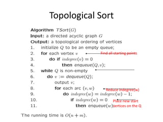


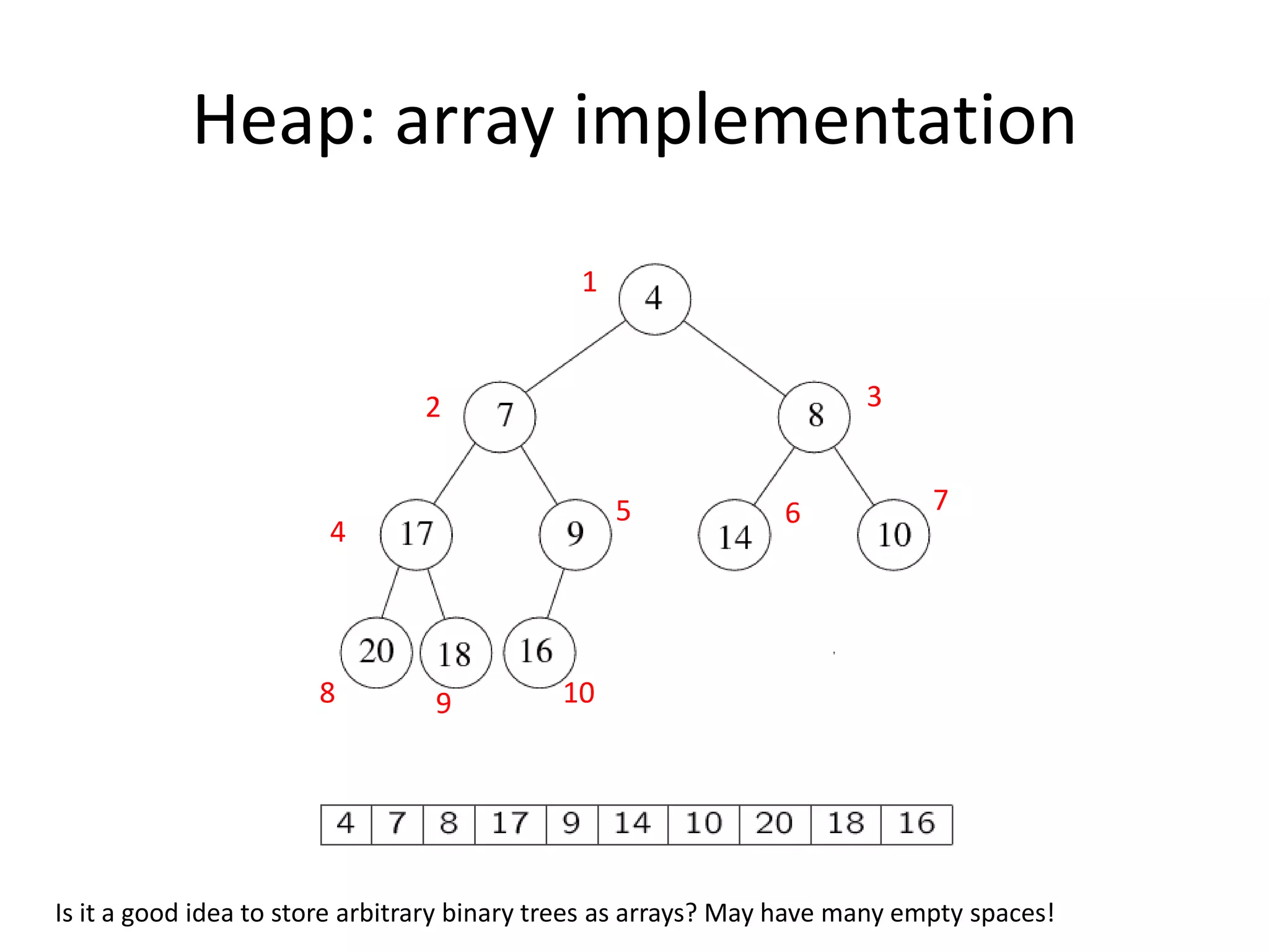
![Array implementation1632514The root node is A[1].The left child of A[j] is A[2j]The right child of A[j] is A[2j + 1]The parent of A[j] is A[j/2] (note: integer divide)25436Need to estimate the maximum size of the heap.](https://image.slidesharecdn.com/sorting2-110225223207-phpapp02/75/Sorting2-5-2048.jpg)


![Counting SortAssume N integers to be sorted, each is in the range 1 to M.Define an array B[1..M], initialize all to 0 O(M)Scan through the input list A[i], insert A[i] into B[A[i]] O(N)Scan B once, read out the nonzero integers O(M)Total time: O(M + N)if M is O(N), then total time is O(N)Can be bad if range is very big, e.g. M=O(N2)N=7, M = 9, Want to sort 8 1 9 5 2 6 3 5893612Output: 1 2 3 5 6 8 9](https://image.slidesharecdn.com/sorting2-110225223207-phpapp02/75/Sorting2-22-2048.jpg)
![Counting sortWhat if we have duplicates?B is an array of pointers.Each position in the array has 2 pointers: head and tail. Tail points to the end of a linked list, and head points to the beginning.A[j] is inserted at the end of the list B[A[j]]Again, Array B is sequentially traversed and each nonempty list is printed out.Time: O(M + N)](https://image.slidesharecdn.com/sorting2-110225223207-phpapp02/75/Sorting2-23-2048.jpg)


![// base 10// FIFO// d times of counting sort// scan A[i], put into correct slot// re-order back to original array](https://image.slidesharecdn.com/sorting2-110225223207-phpapp02/75/Sorting2-31-2048.jpg)

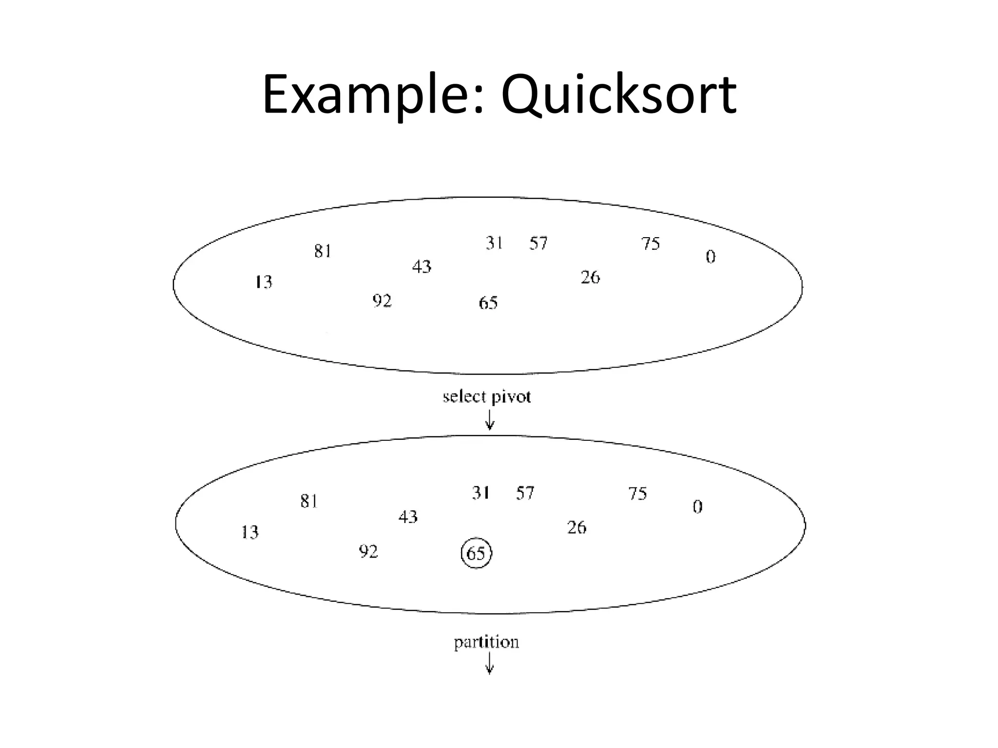
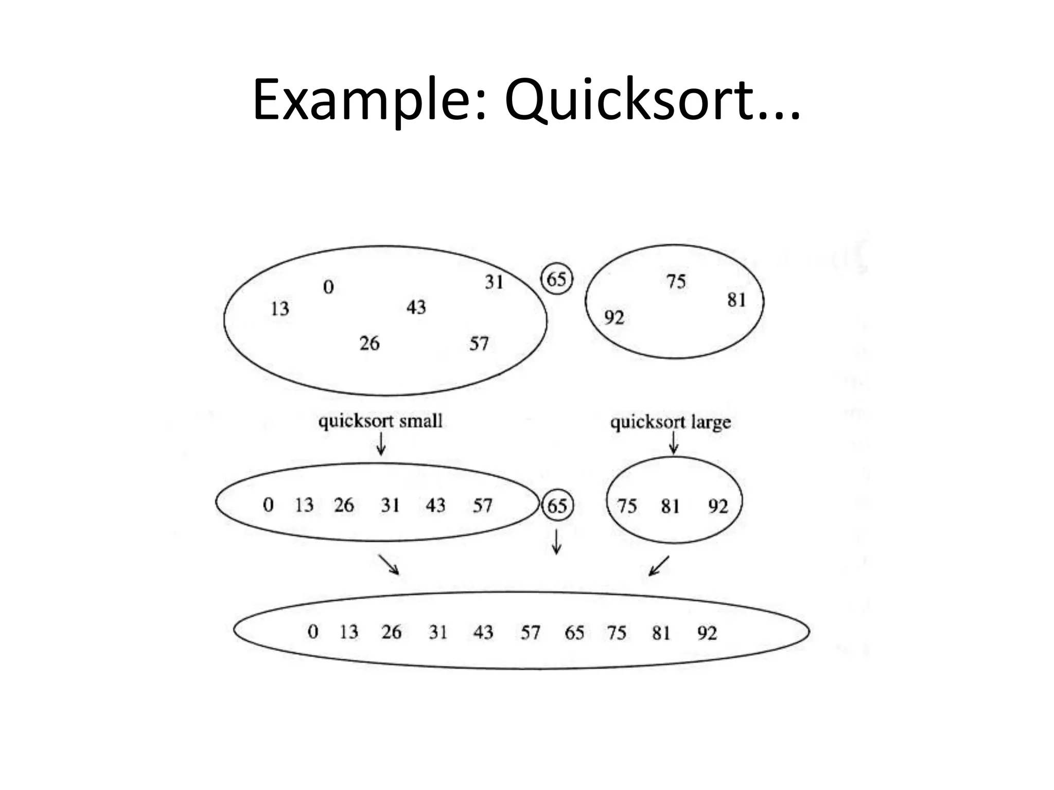
![Pseudocode Input: an array A[p, r]Quicksort (A, p, r) { if (p < r) { q = Partition (A, p, r) //q is the position of the pivot elementQuicksort (A, p, q-1)Quicksort (A, q+1, r) }}](https://image.slidesharecdn.com/sorting2-110225223207-phpapp02/75/Sorting2-38-2048.jpg)

![Partitioning Strategy196jiWant to partition an array A[left .. right]First, get the pivot element out of the way by swapping it with the last element. (Swap pivot and A[right])Let i start at the first element and j start at the next-to-last element (i = left, j = right – 1)swap656431219564312pivot](https://image.slidesharecdn.com/sorting2-110225223207-phpapp02/75/Sorting2-40-2048.jpg)
![Partitioning Strategy191966jjiiWant to haveA[p] <= pivot, for p < iA[p] >= pivot, for p > jWhen i < jMove i right, skipping over elements smaller than the pivotMove j left, skipping over elements greater than the pivotWhen both i and j have stoppedA[i] >= pivotA[j] <= pivot564312564312](https://image.slidesharecdn.com/sorting2-110225223207-phpapp02/75/Sorting2-41-2048.jpg)
![Partitioning Strategy191966jjiiWhen i and j have stopped and i is to the left of jSwap A[i] and A[j]The large element is pushed to the right and the small element is pushed to the leftAfter swappingA[i] <= pivotA[j] >= pivotRepeat the process until i and j crossswap564312534612](https://image.slidesharecdn.com/sorting2-110225223207-phpapp02/75/Sorting2-42-2048.jpg)
![Partitioning Strategy191919666jjjiiiWhen i and j have crossedSwap A[i] and pivotResult:A[p] <= pivot, for p < iA[p] >= pivot, for p > i534612534612534612](https://image.slidesharecdn.com/sorting2-110225223207-phpapp02/75/Sorting2-43-2048.jpg)


![Pivot: median of threeWe will use median of threeCompare just three elements: the leftmost, rightmost and centerSwap these elements if necessary so that A[left] = SmallestA[right] = LargestA[center] = Median of threePick A[center] as the pivotSwap A[center] and A[right – 1] so that pivot is at second last position (why?)median3](https://image.slidesharecdn.com/sorting2-110225223207-phpapp02/75/Sorting2-47-2048.jpg)
![66521365261352135213pivotpivot19Pivot: median of threeA[left] = 2, A[center] = 13, A[right] = 66431219Swap A[center] and A[right]64312196431219Choose A[center] as pivotSwap pivot and A[right – 1]64312Note we only need to partition A[left + 1, …, right – 2]. Why?](https://image.slidesharecdn.com/sorting2-110225223207-phpapp02/75/Sorting2-48-2048.jpg)
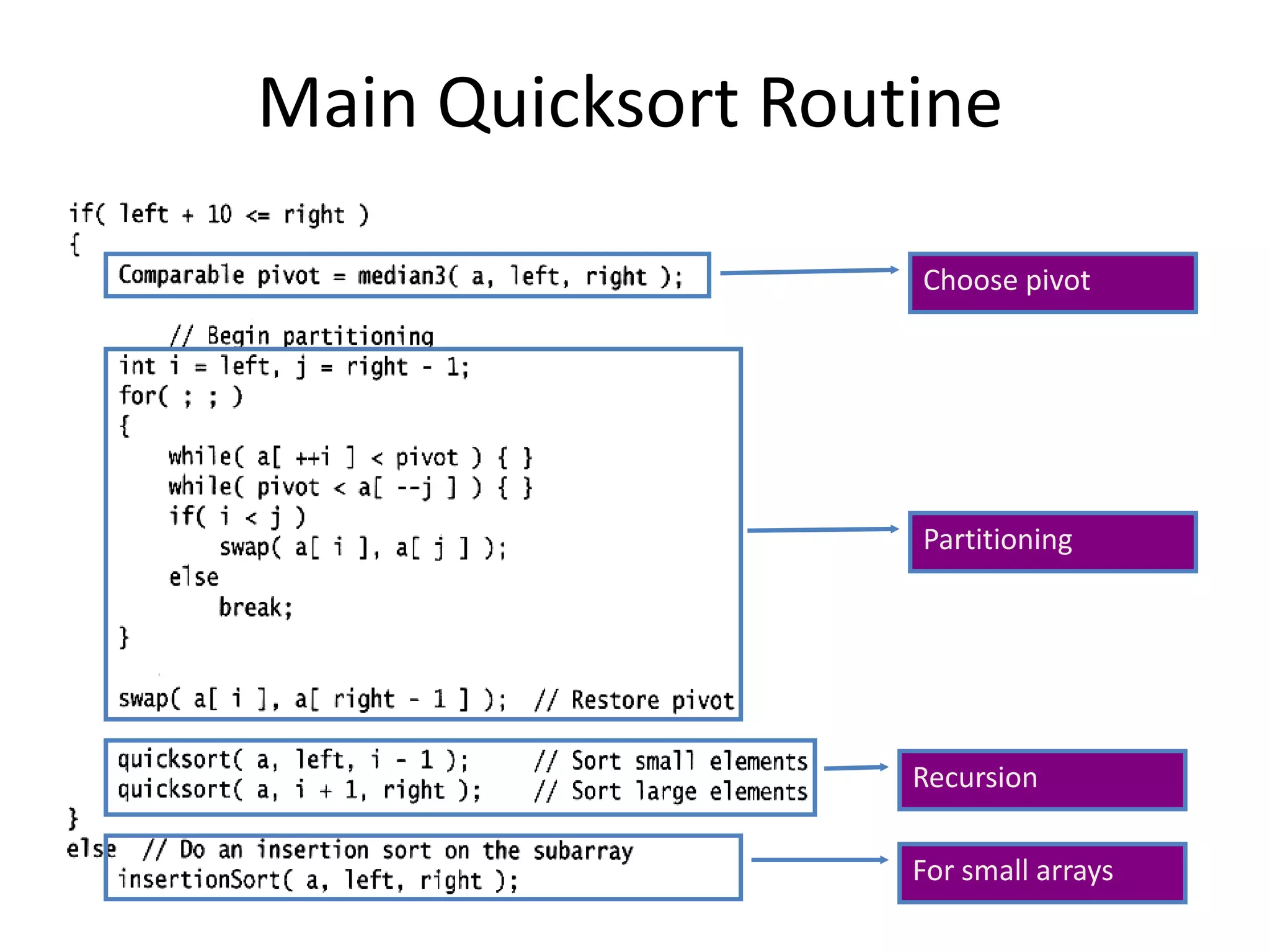
![Partitioning PartWorks only if pivot is picked as median-of-three. A[left] <= pivot and A[right] >= pivotThus, only need to partition A[left + 1, …, right – 2]j will not run past the endbecause a[left] <= pivoti will not run past the endbecause a[right-1] = pivot](https://image.slidesharecdn.com/sorting2-110225223207-phpapp02/75/Sorting2-50-2048.jpg)
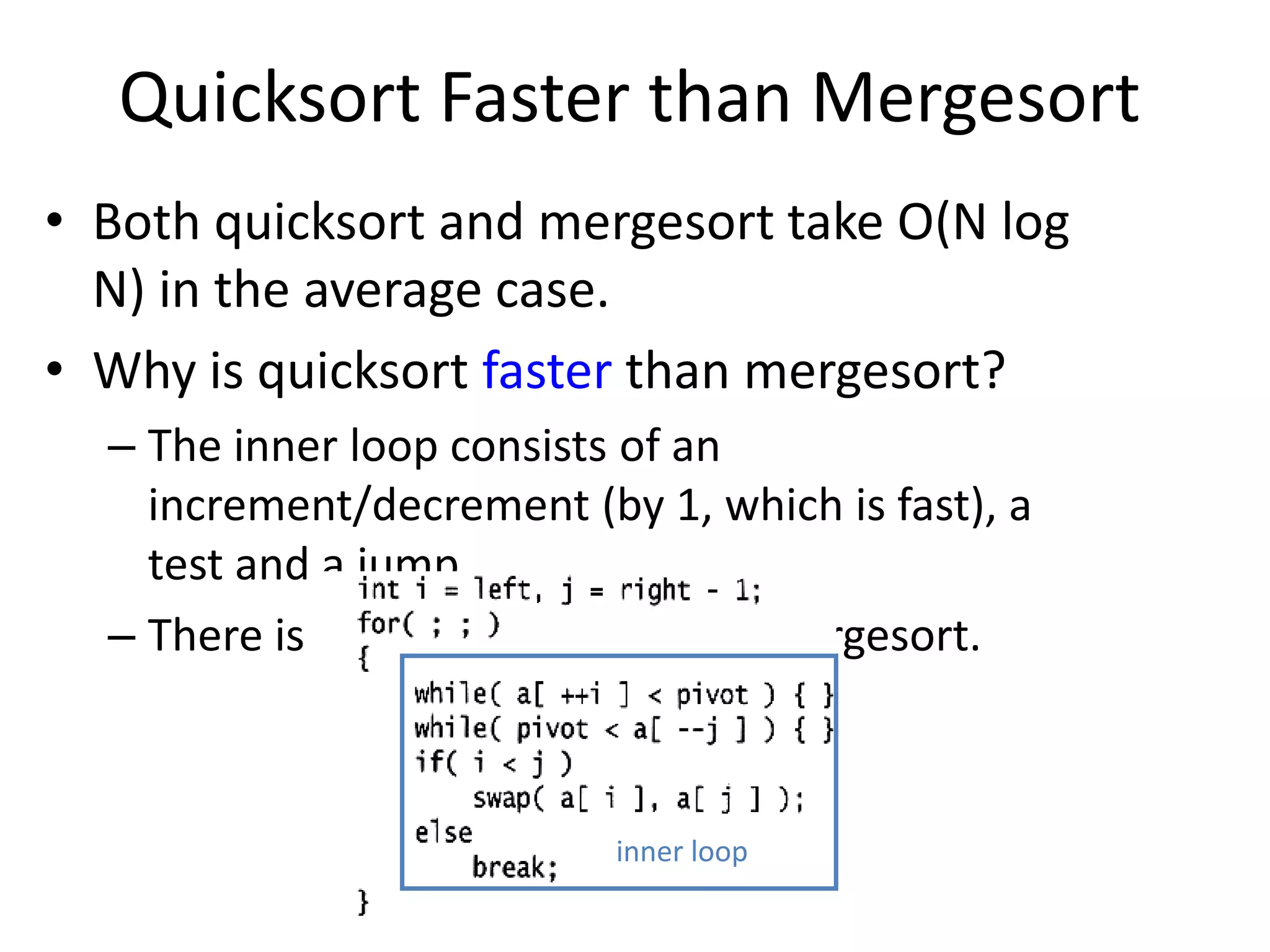
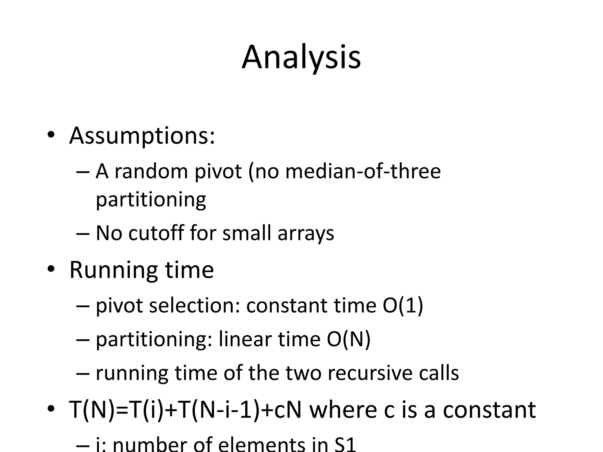


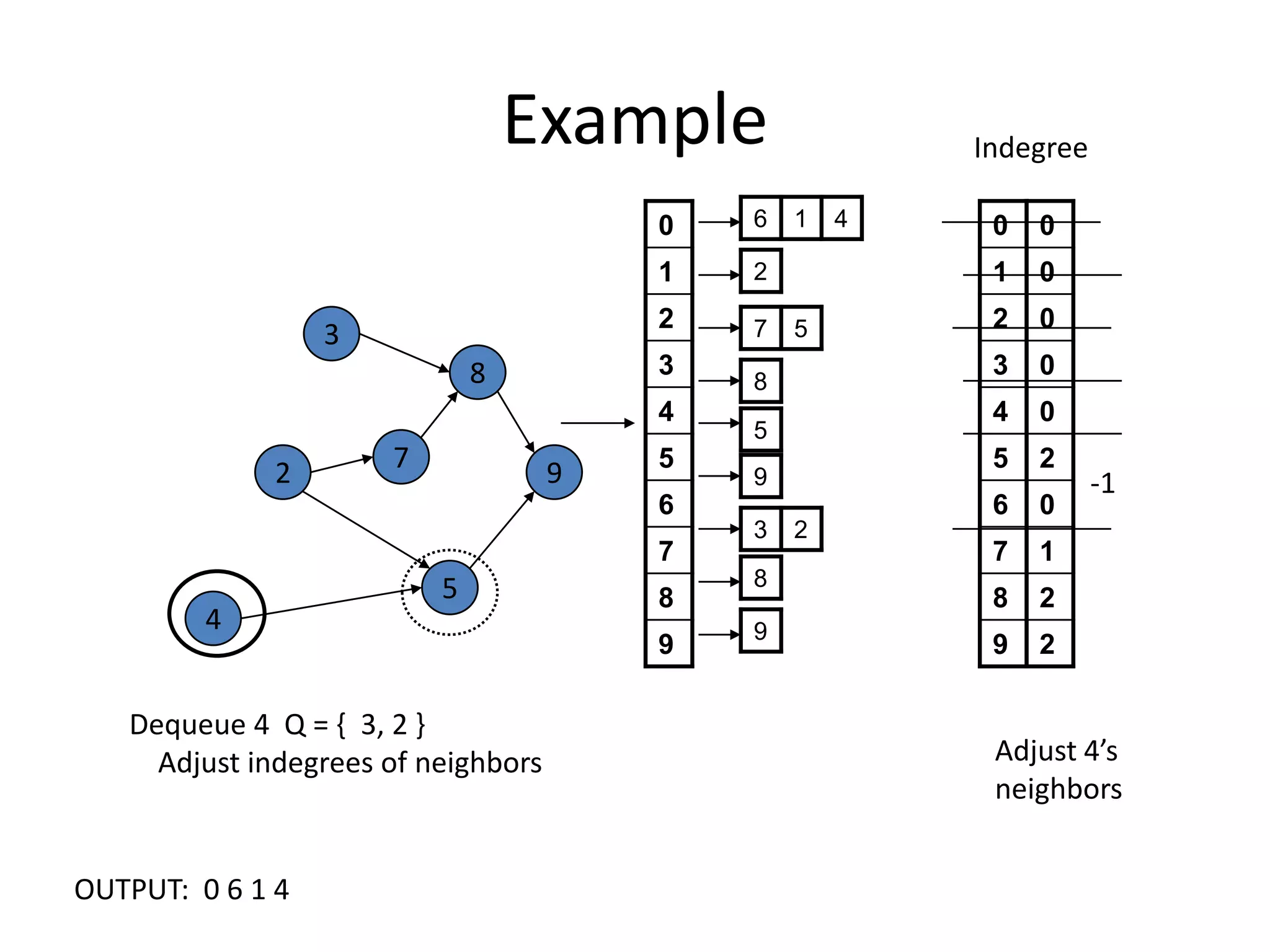

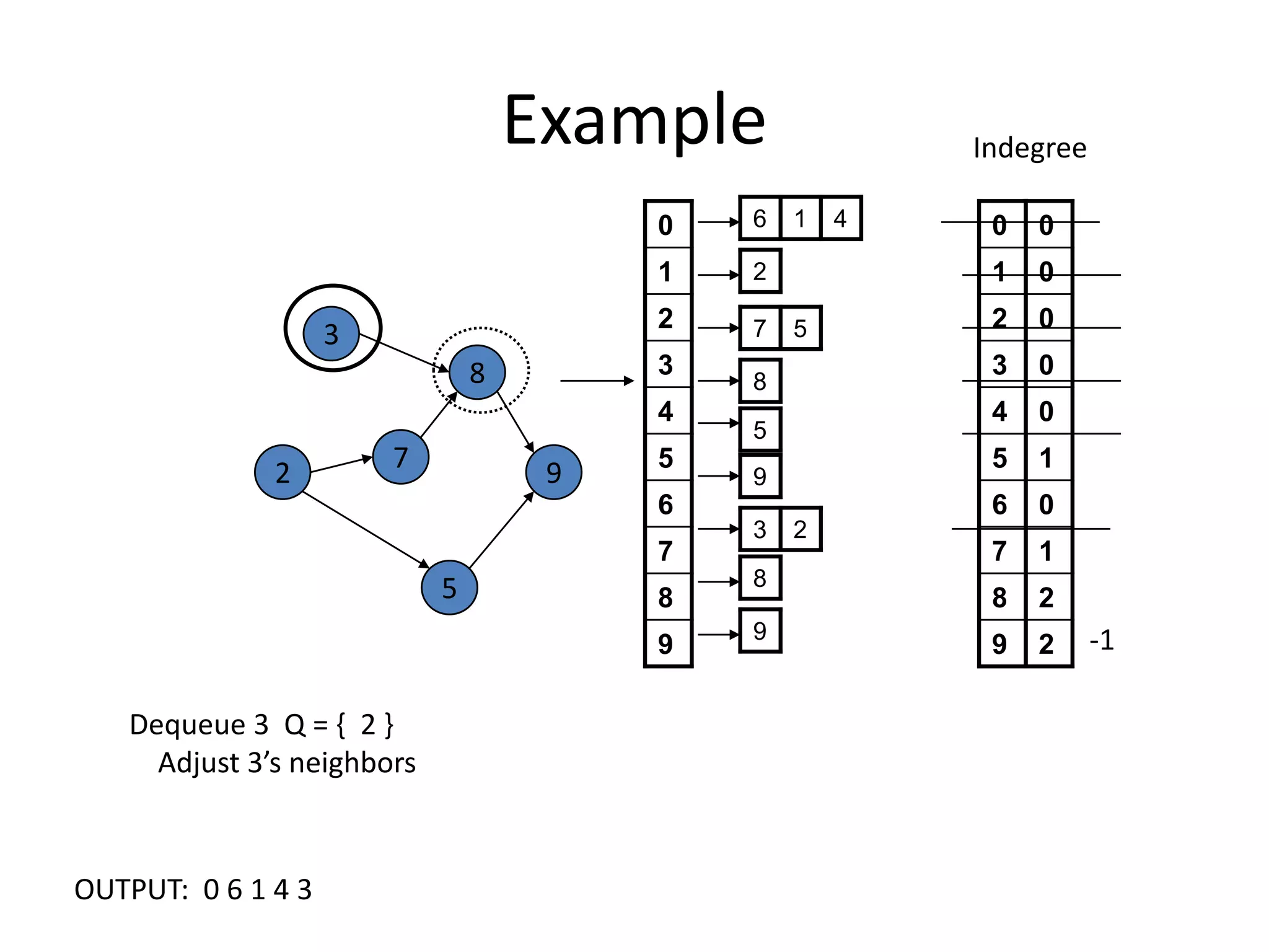
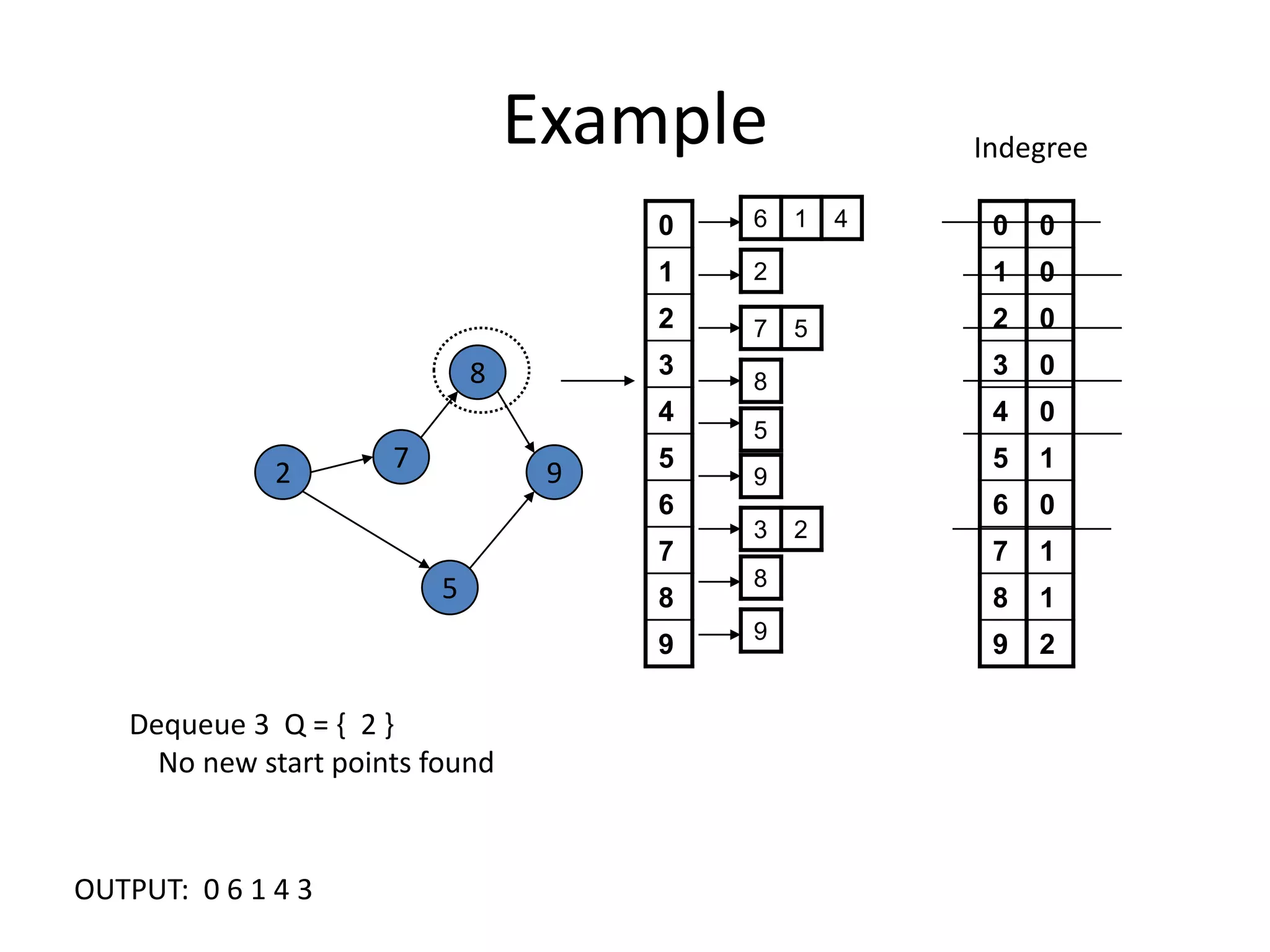
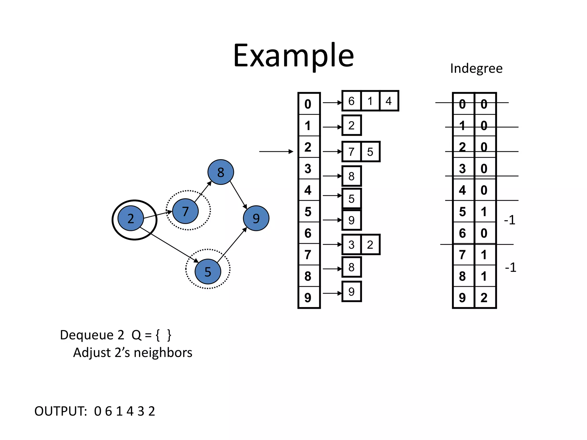


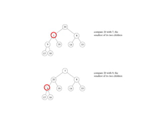
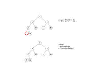
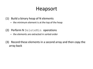
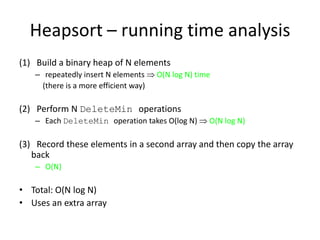
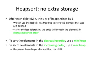
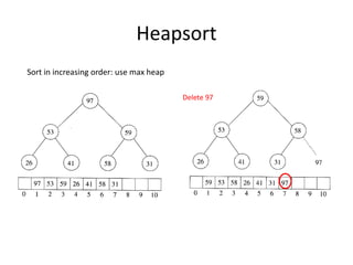
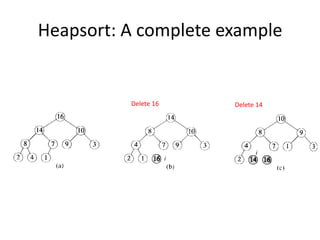
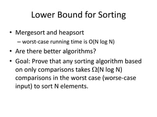
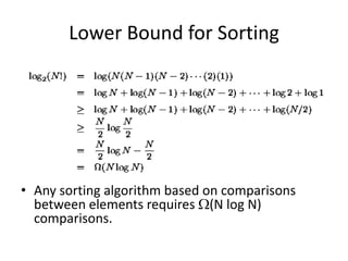
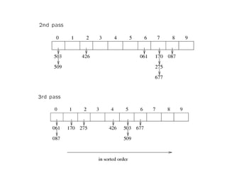
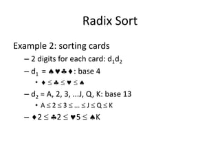
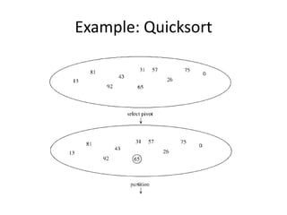
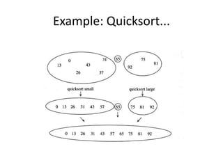
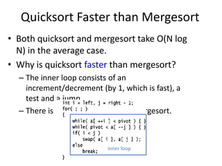
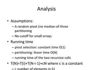
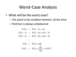
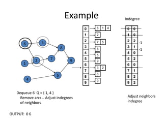
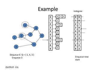
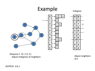
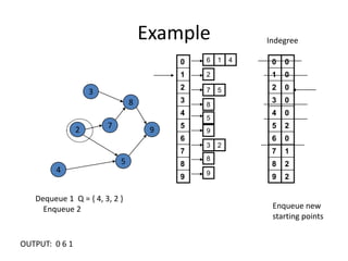
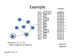
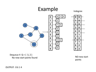
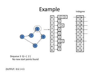
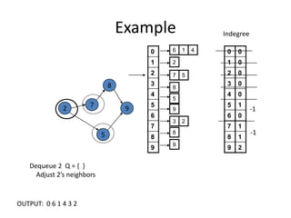
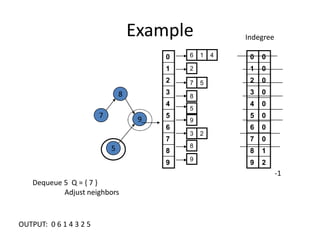
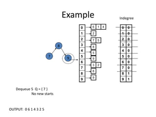
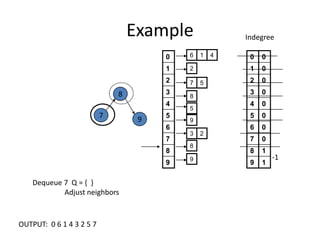
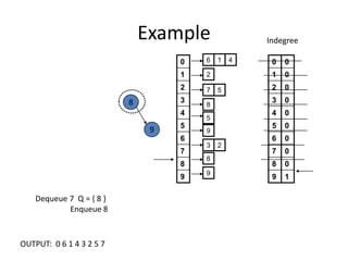
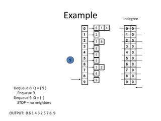
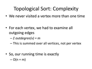
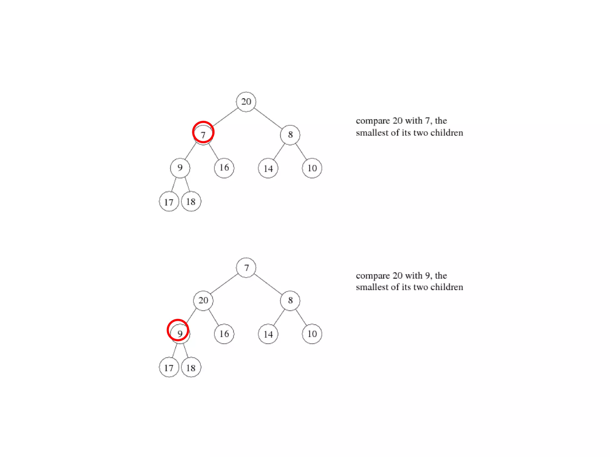
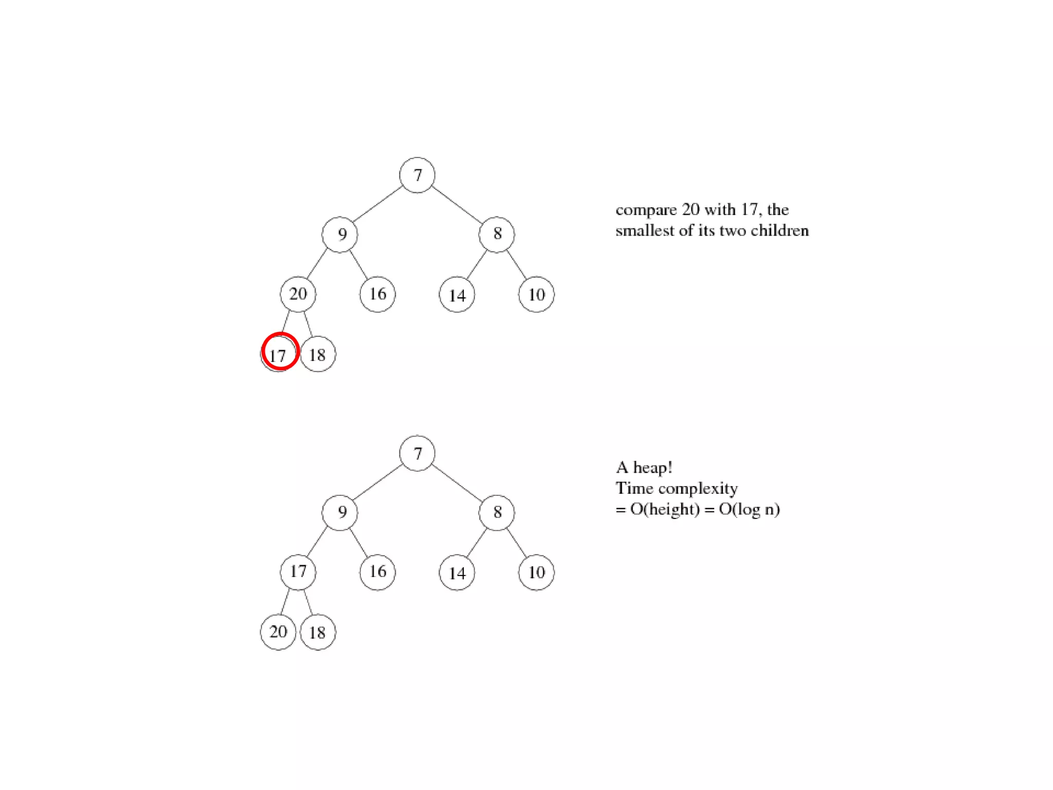
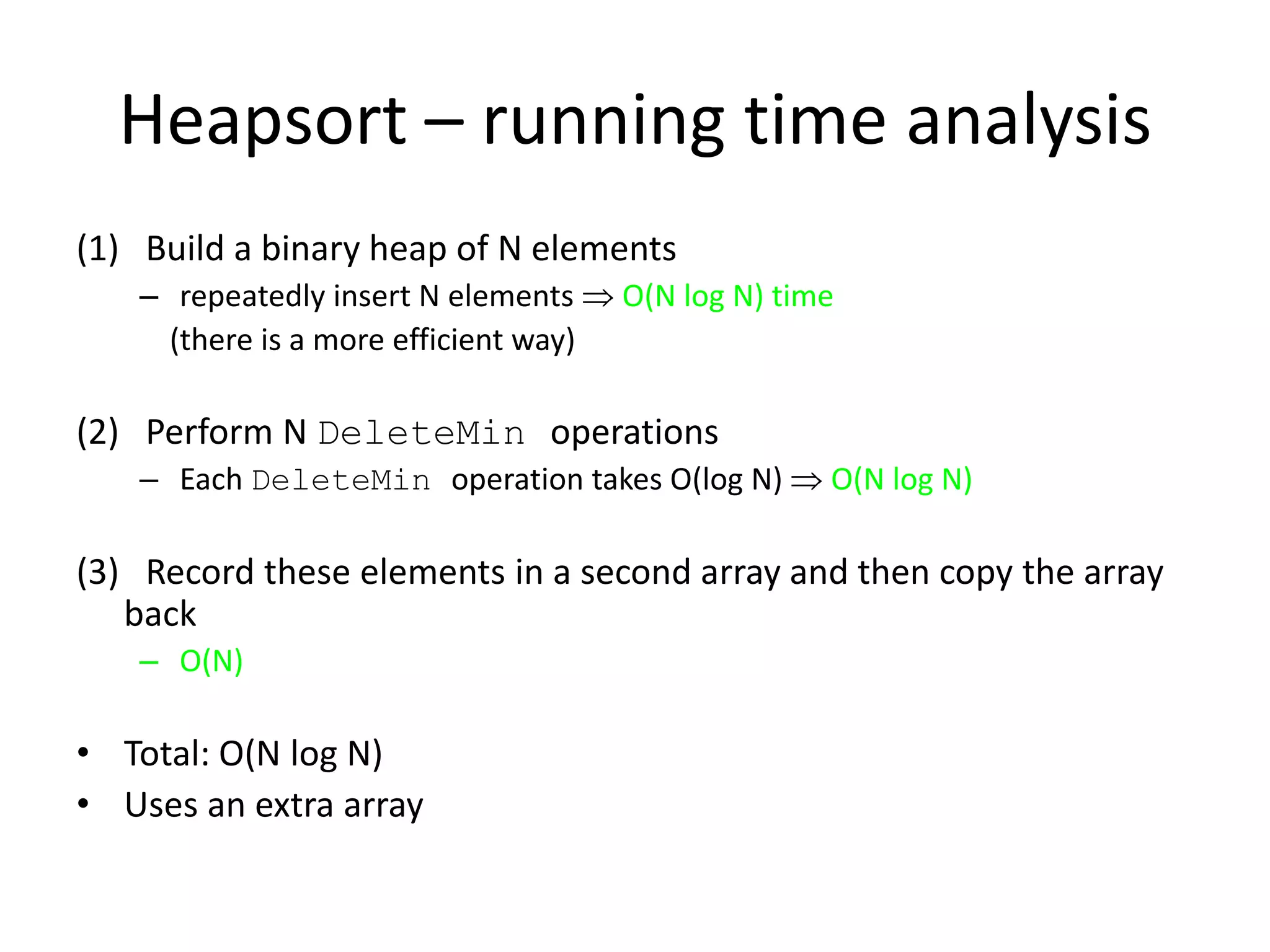
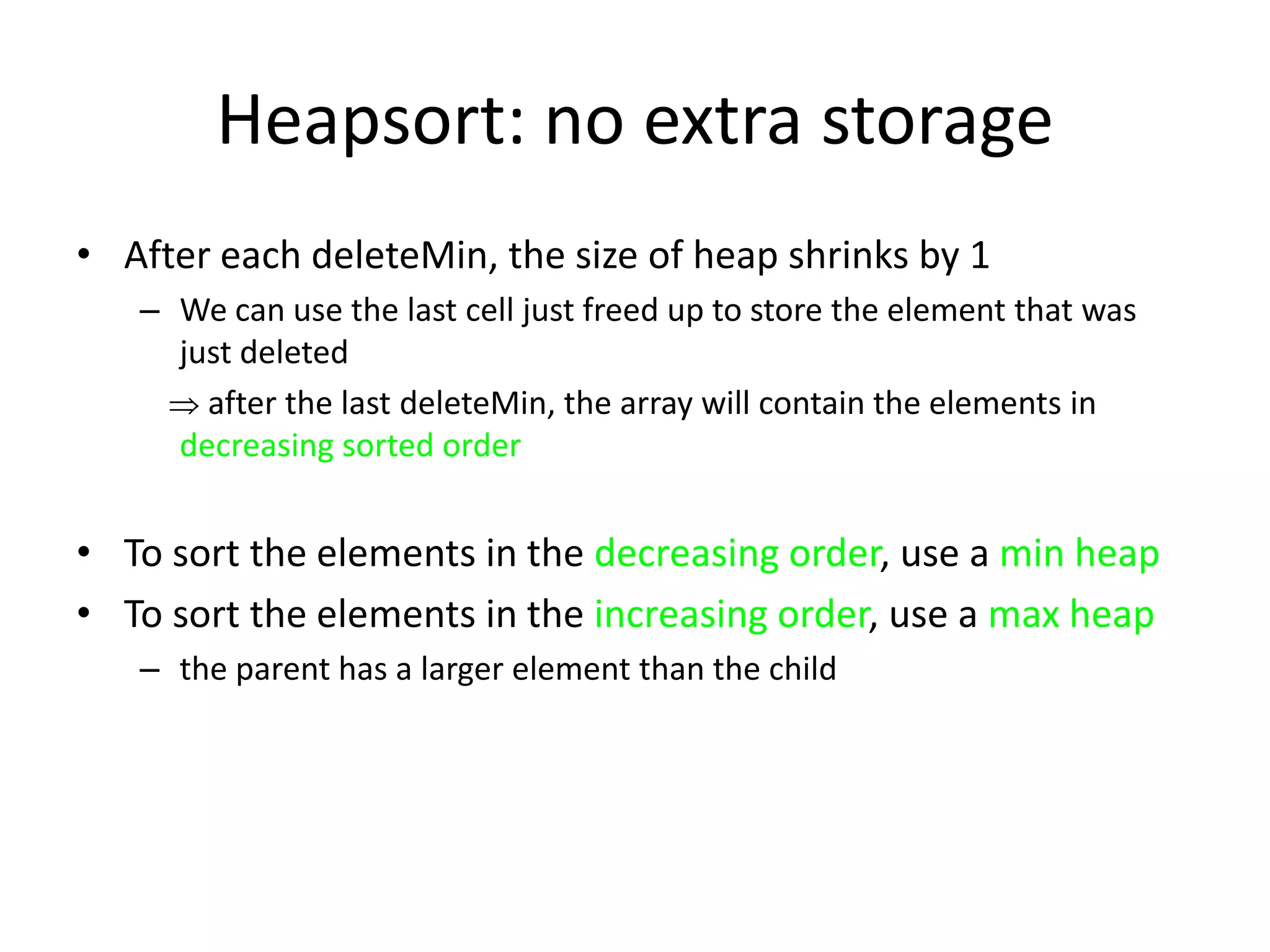
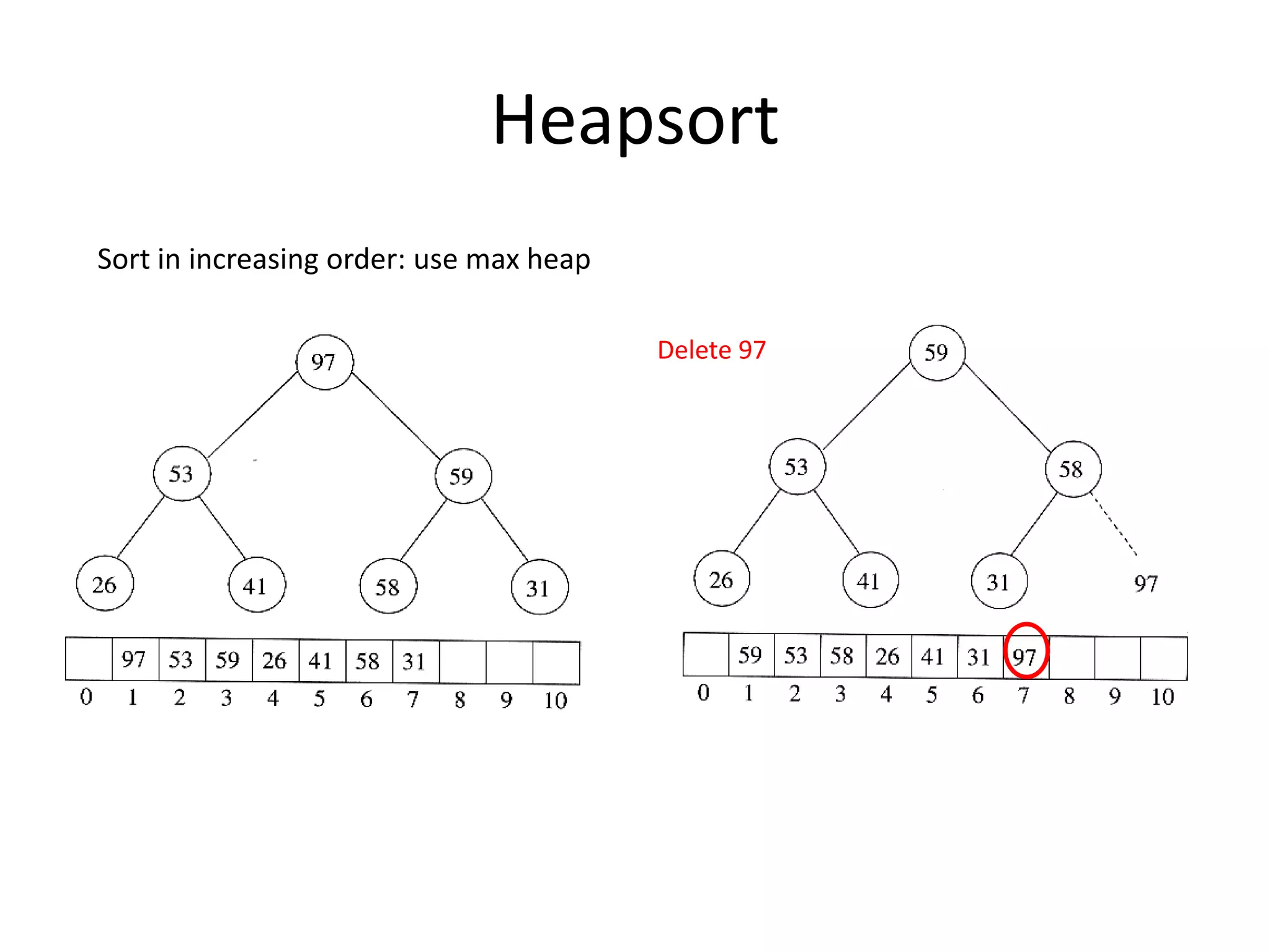
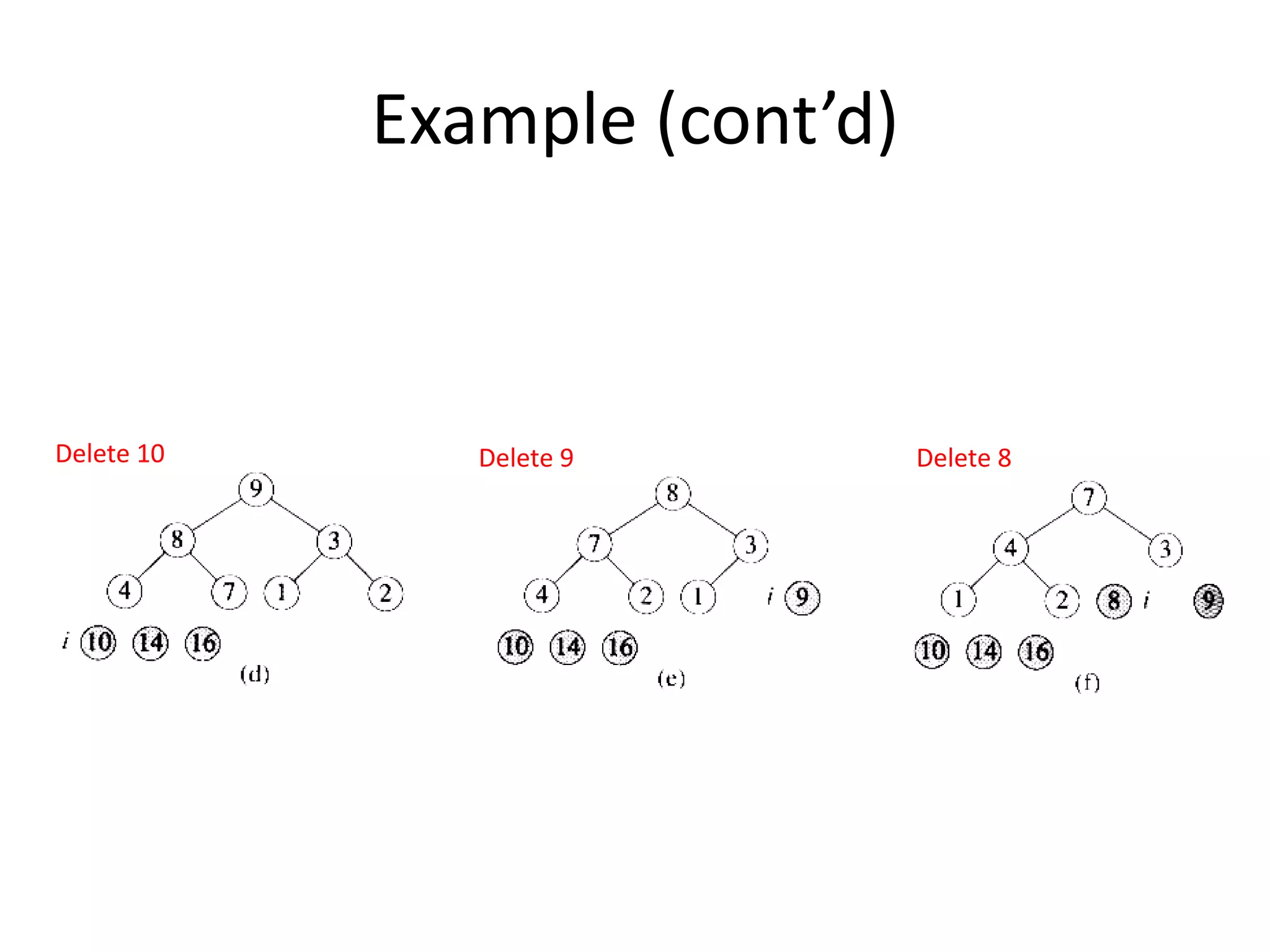
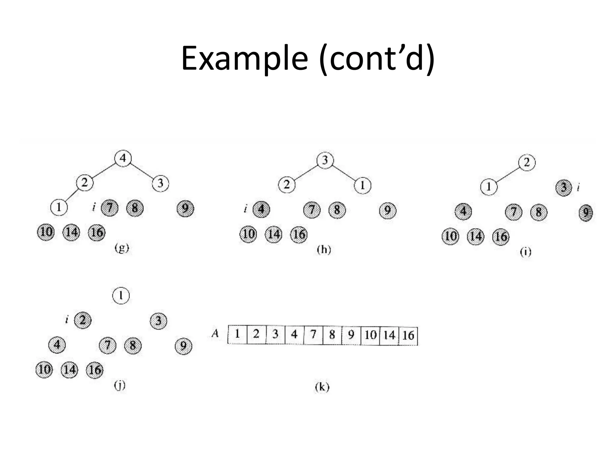
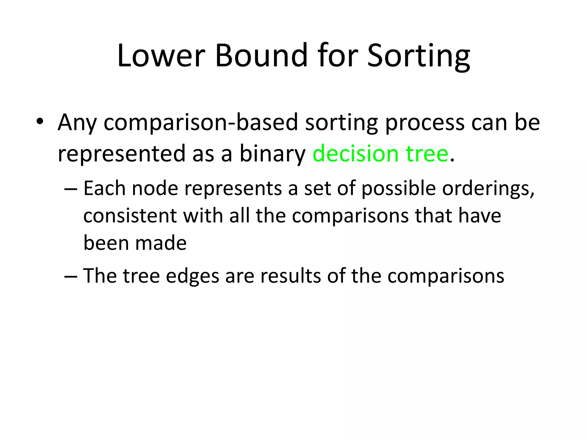
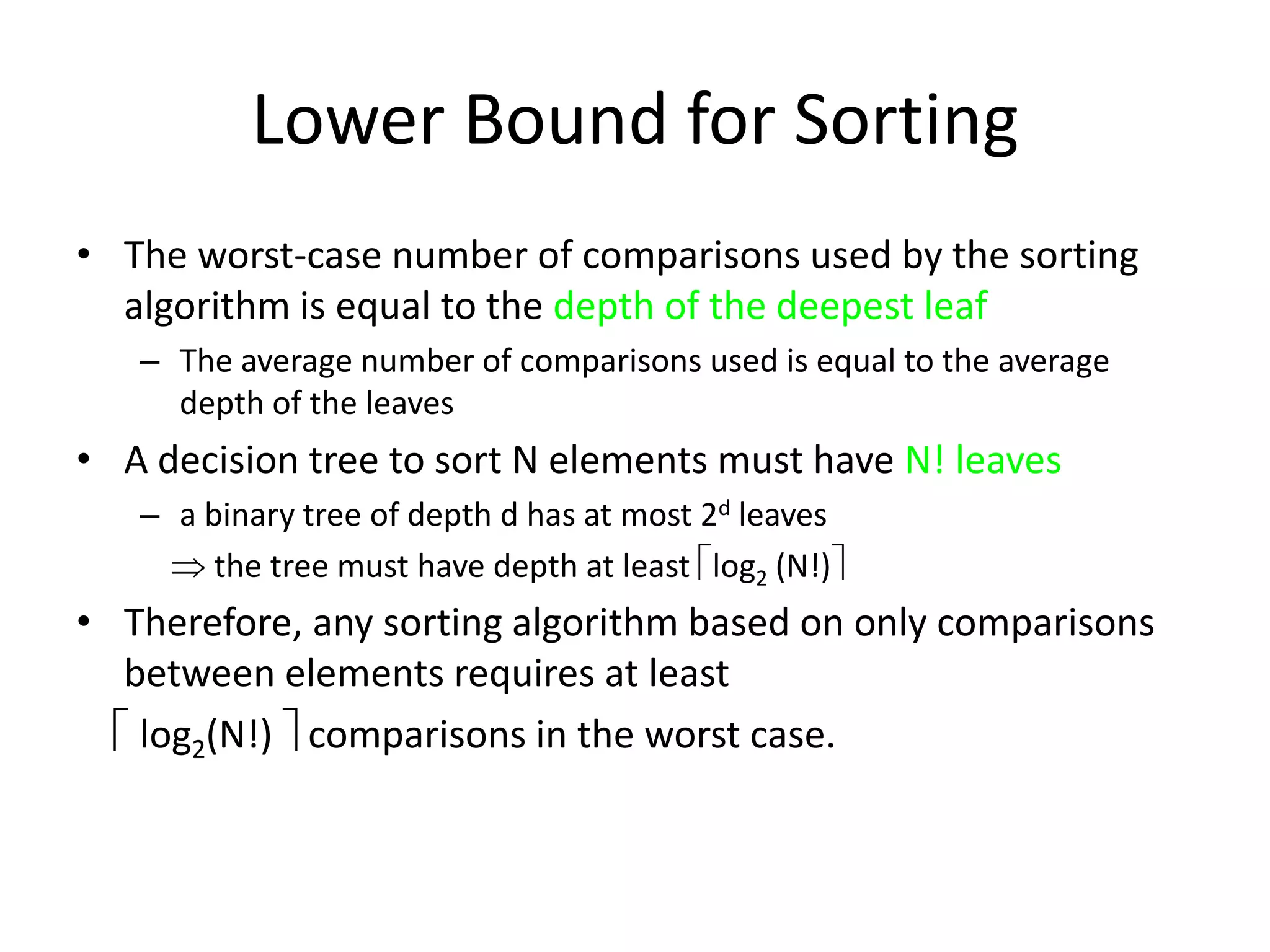
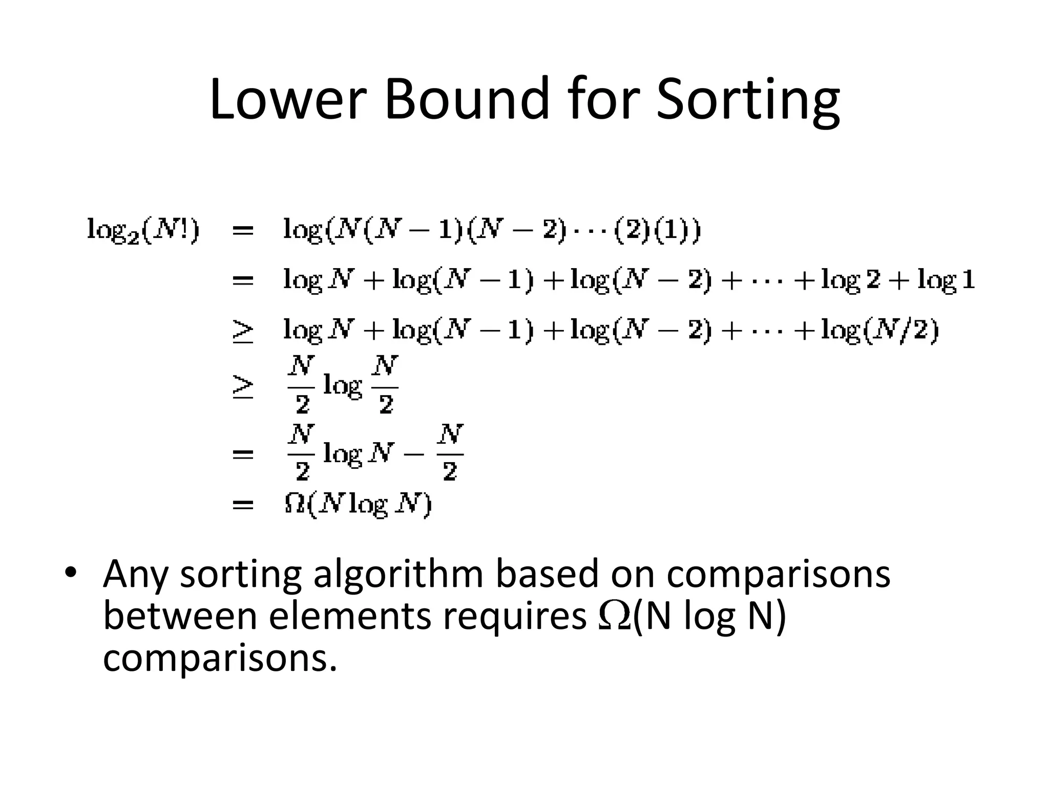
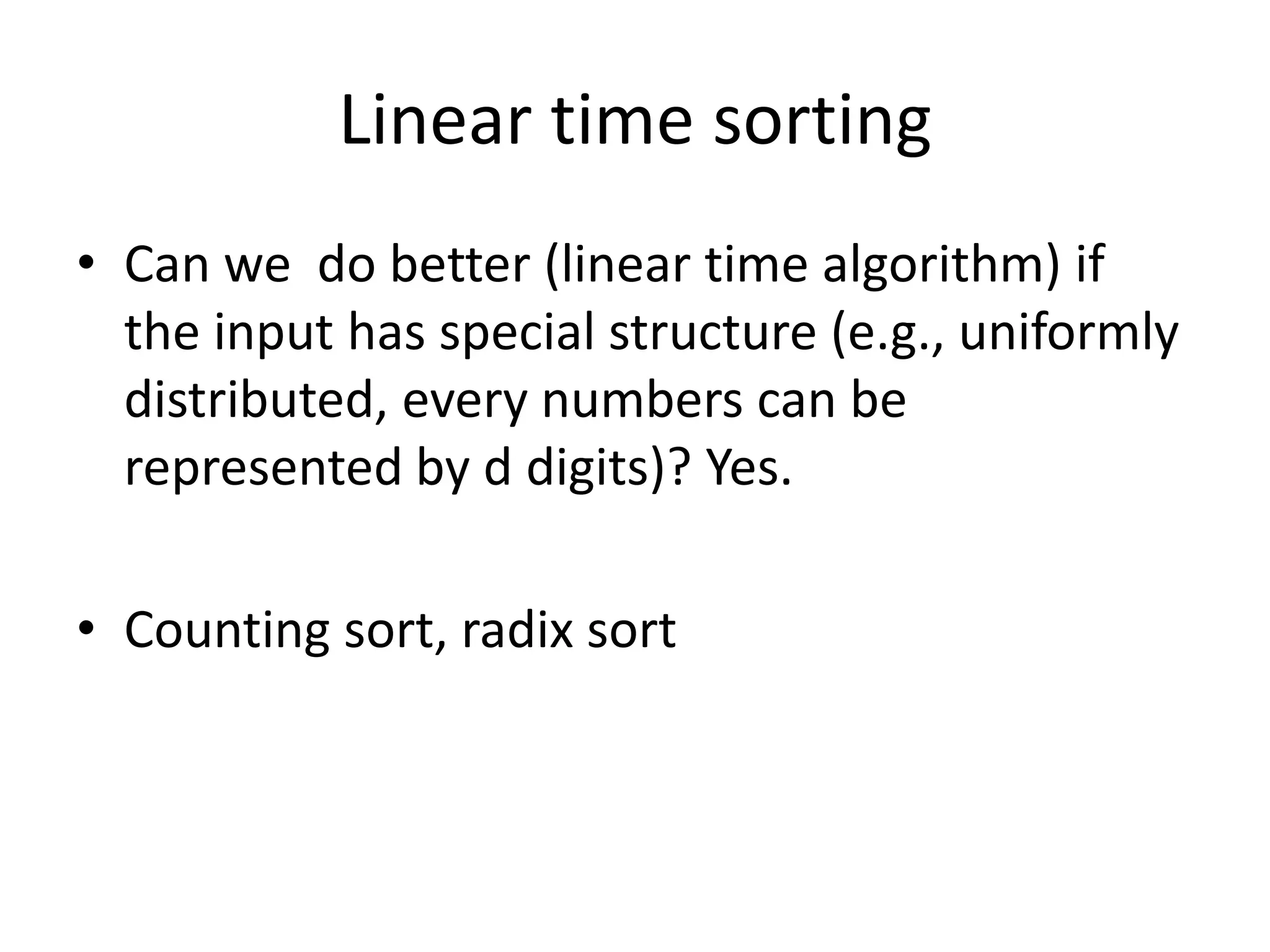
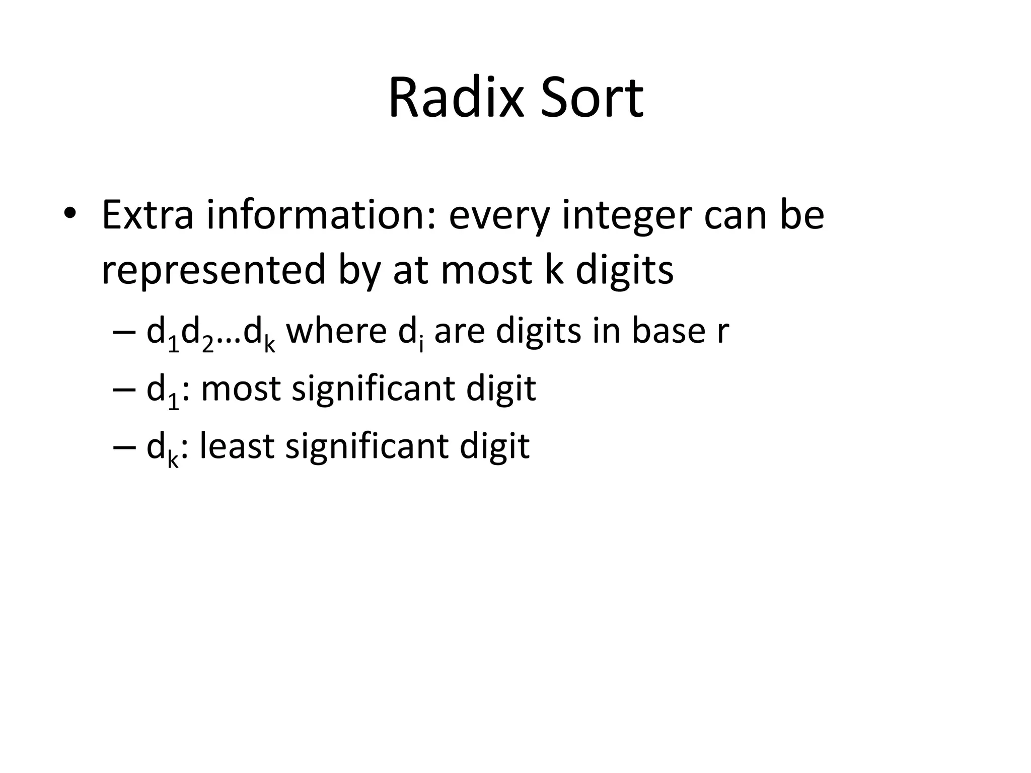
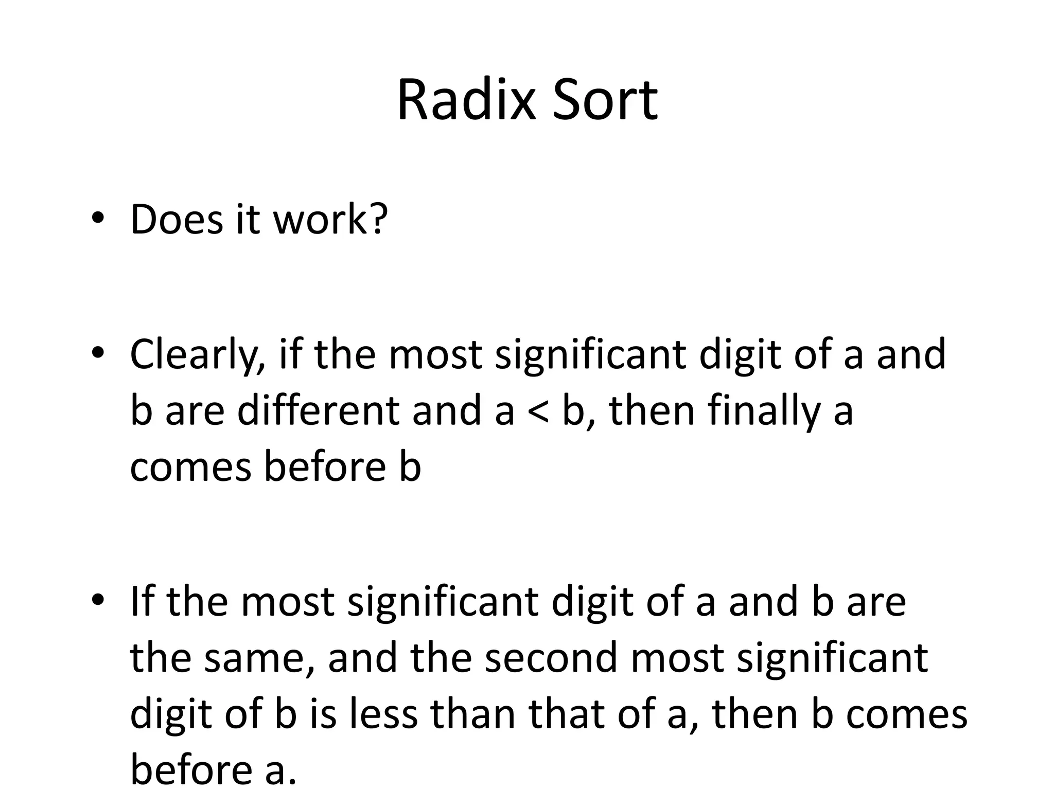
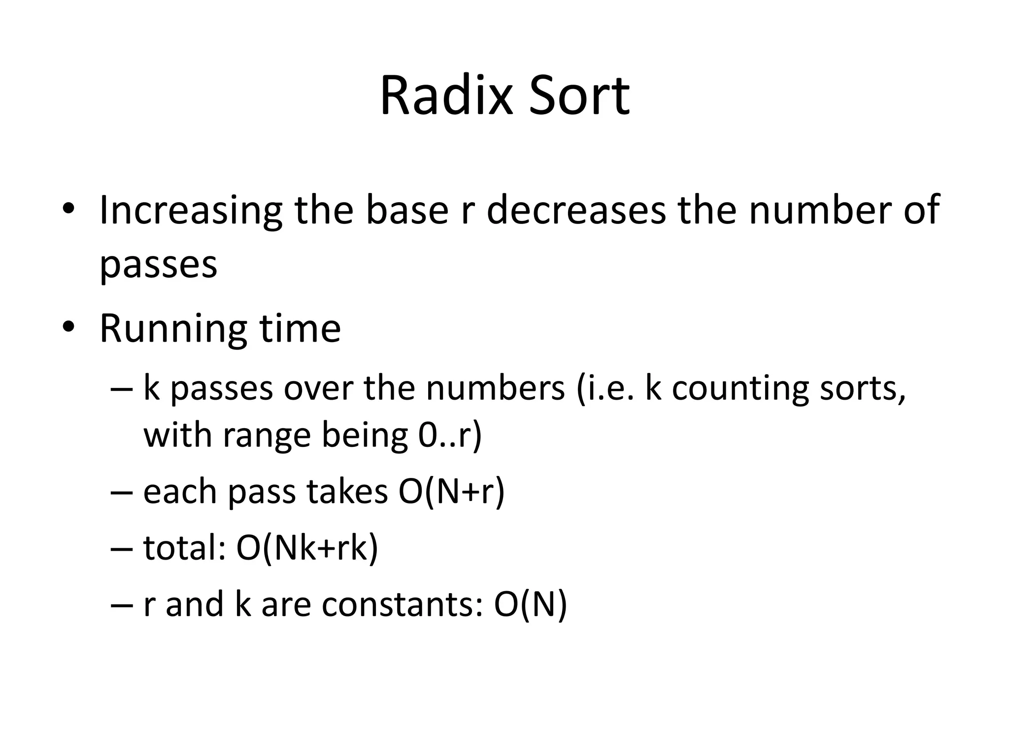
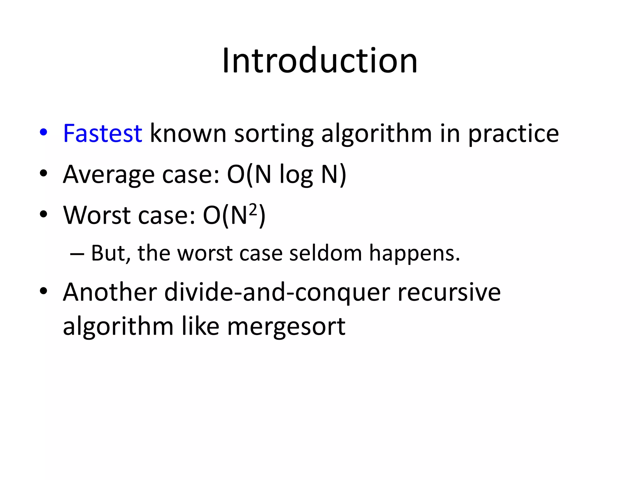
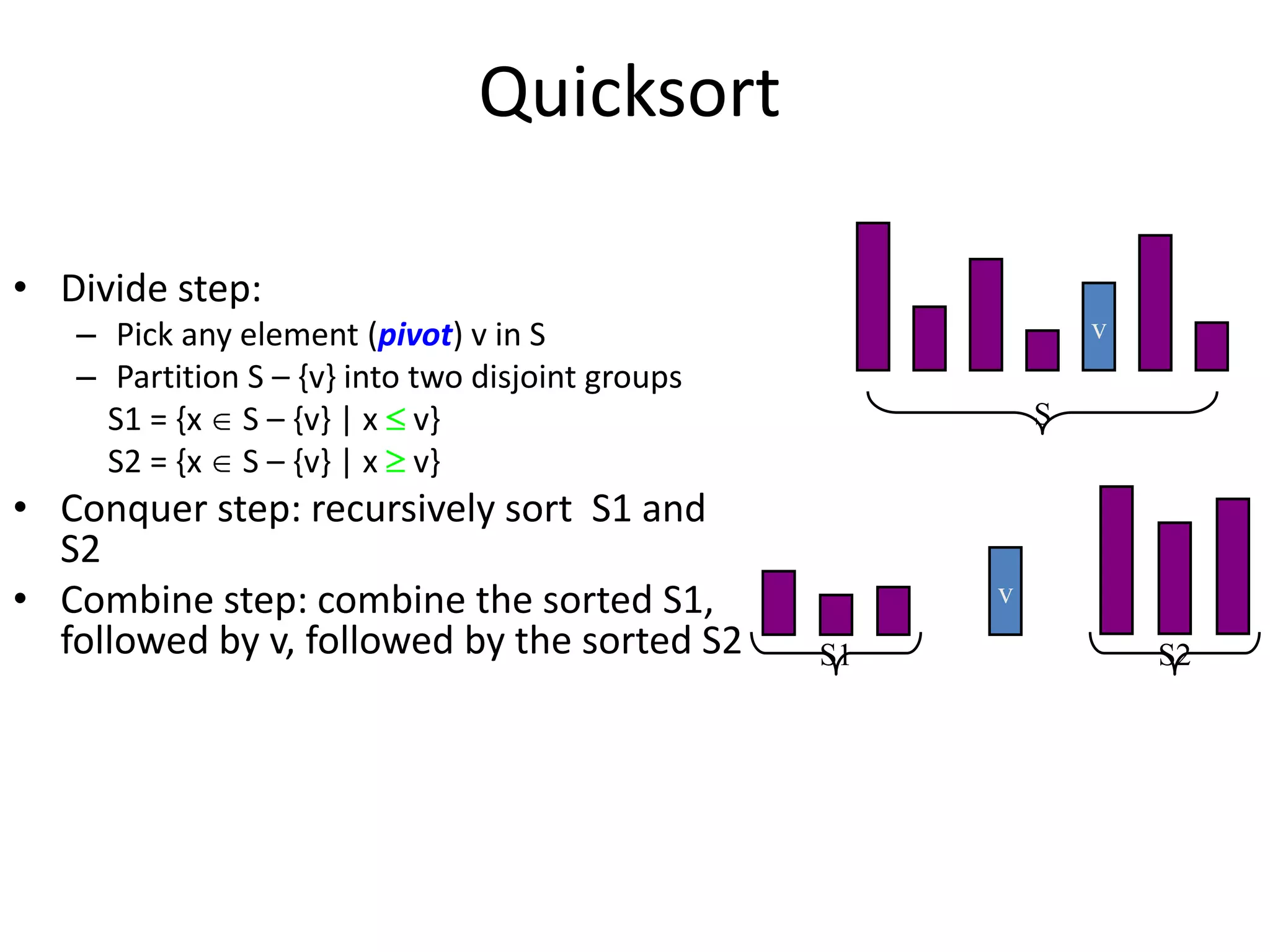
The document discusses various sorting algorithms and their time complexities, including: 1) Quicksort, which has an average case time complexity of O(n log n) but a worst case of O(n^2). It works by recursively partitioning an array around a pivot element. 2) Heapsort, which also has a time complexity of O(n log n). It uses a binary heap to extract elements in sorted order. 3) Counting sort and radix sort, which can sort in linear time O(n) when the input has certain properties like a limited range of values or being represented by a small number of digits.


![UNIT V Searching Sorting Hashing Techniques [Autosaved].pptx](https://cdn.slidesharecdn.com/ss_thumbnails/unitvsearchingsortinghashingtechniquesautosaved-241126054304-95a69c51-thumbnail.jpg?width=600ounds&width=560&fit=bounds)
![UNIT V Searching Sorting Hashing Techniques [Autosaved].pptx](https://cdn.slidesharecdn.com/ss_thumbnails/unitvsearchingsortinghashingtechniquesautosaved-241014040608-74caa0f6-thumbnail.jpg?width=600ounds&width=560&fit=bounds)


![UiPath Automation Suite Installation (Hands-On) [2/3]](https://cdn.slidesharecdn.com/ss_thumbnails/automationsuitecommunitysession2-251015095633-a6d862f1-thumbnail.jpg?width=600ounds&width=560&fit=bounds)


