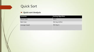
Quicksort is a recursive divide-and-conquer algorithm that works by selecting a pivot element and partitioning the array into two subarrays of elements less than and greater than the pivot. It recursively sorts the subarrays. The divide step does all the work by partitioning, while the combine step does nothing. It has average case performance of O(n log n) but worst case of O(n^2). Bubble sort repeatedly swaps adjacent elements that are out of order until the array is fully sorted. It has a simple implementation but poor performance of O(n^2).
Quick Sort
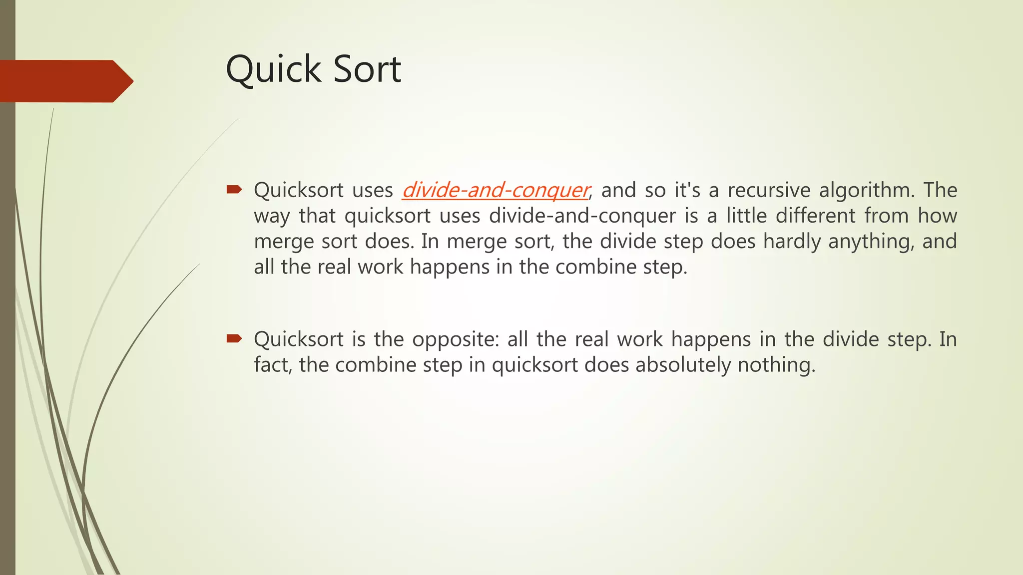
Quicksortuses divide-and-conquer, and so it's a recursive algorithm. The
way that quicksort uses divide-and-conquer is a little different from how
merge sort does. In merge sort, the divide step does hardly anything, and
all the real work happens in the combine step.
Quicksort is the opposite: all the real work happens in the divide step. In
fact, the combine step in quicksort does absolutely nothing.
3.
Quick Sort
Hereis how quicksort uses divide-and-conquer: think of sorting a sub
array[p…r], Where initially the sub array is array[0…n-1].
We take this set of array as an example:
40 20 10 80 60 50 7 30 100
0 1 2 3 4 5 6 7 8
4.
Quick Sort
Divide
1.Choose any element in the sub array [p…r] call this element Pivot.
We now have our Pivot which is 40 at array 0
40 20 10 80 60 50 7 30 100
0 1 2 3 4 5 6 7 8
5.
Quick Sort
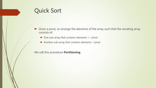
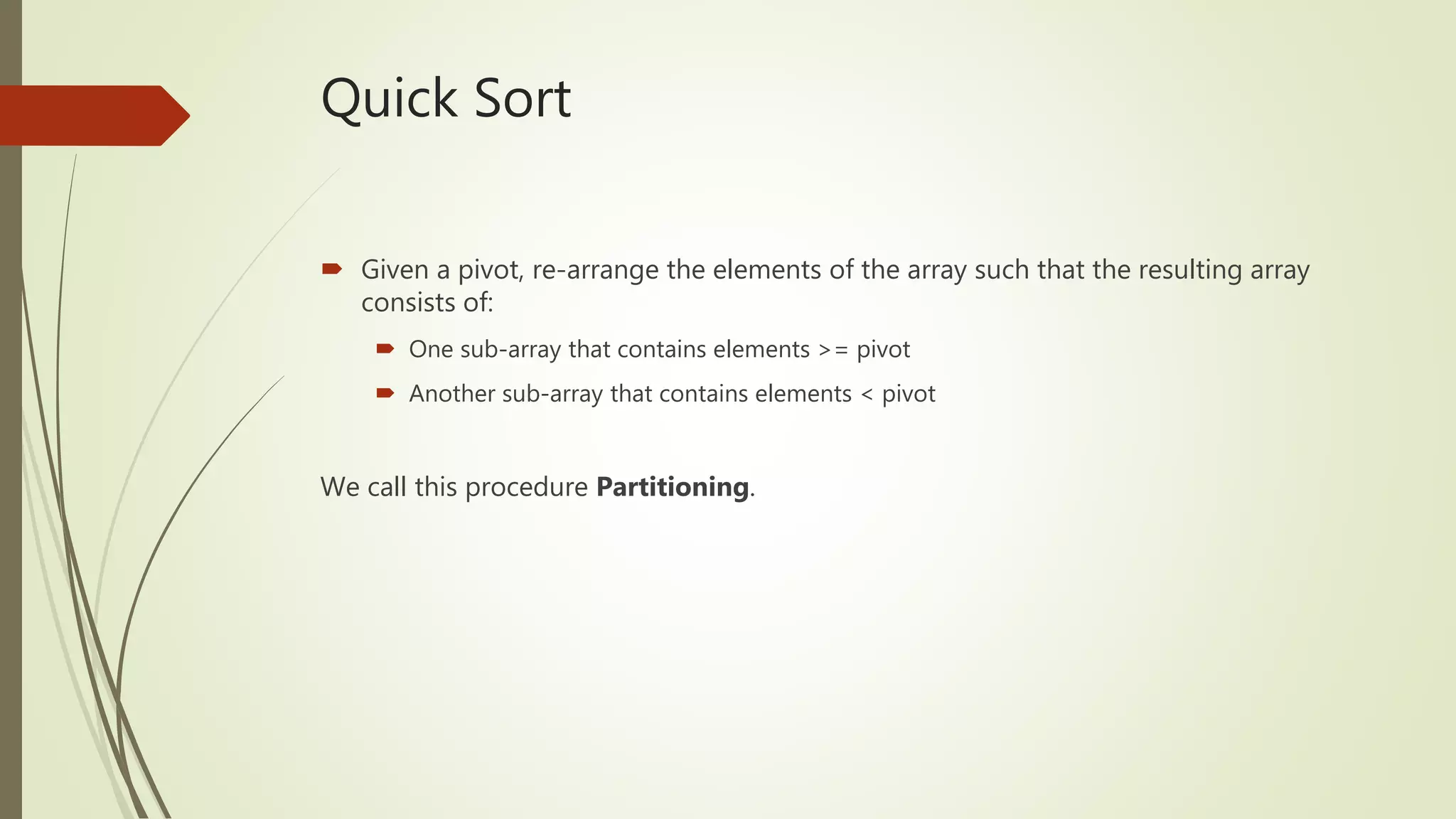
Givena pivot, re-arrange the elements of the array such that the resulting array
consists of:
One sub-array that contains elements >= pivot
Another sub-array that contains elements < pivot
We call this procedure Partitioning.
Quick Sort
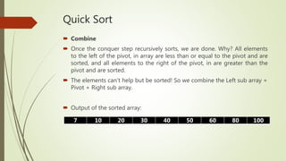
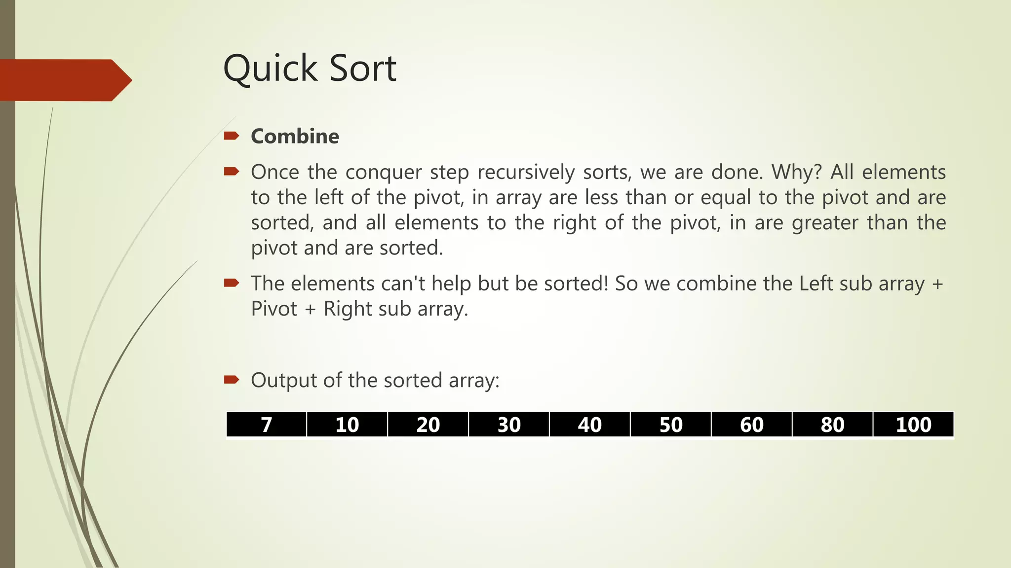
Combine
Once the conquer step recursively sorts, we are done. Why? All elements
to the left of the pivot, in array are less than or equal to the pivot and are
sorted, and all elements to the right of the pivot, in are greater than the
pivot and are sorted.
The elements can't help but be sorted! So we combine the Left sub array +
Pivot + Right sub array.
Output of the sorted array:
7 10 20 30 40 50 60 80 100
Quick Sort
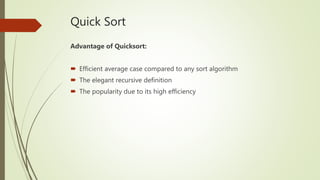
Advantage ofQuicksort:
Efficient average case compared to any sort algorithm
The elegant recursive definition
The popularity due to its high efficiency
12.
Quick Sort
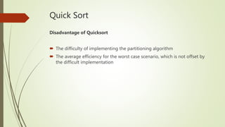
Disadvantage ofQuicksort
The difficulty of implementing the partitioning algorithm
The average efficiency for the worst case scenario, which is not offset by
the difficult implementation
Bubble Sort
Thebubble sort makes multiple passes through a list. It compares adjacent items
and exchanges those that are out of order. Each pass through the list places the
next largest value in its proper place. In essence, each item “bubbles” up to the
location where it belongs.
15.
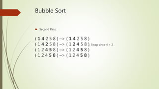
Bubble Sort
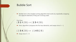
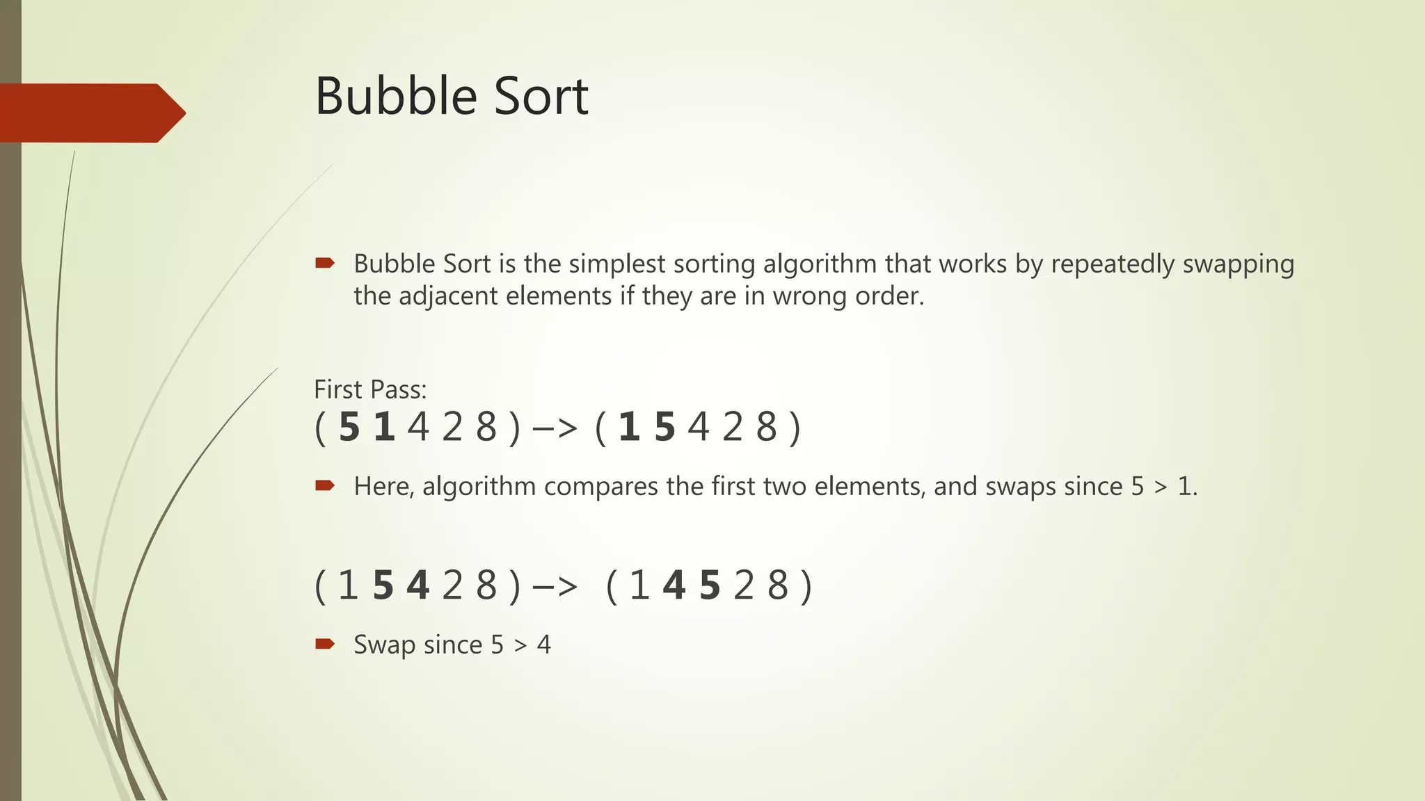
BubbleSort is the simplest sorting algorithm that works by repeatedly swapping
the adjacent elements if they are in wrong order.
First Pass:
( 5 1 4 2 8 ) –> ( 1 5 4 2 8 )
Here, algorithm compares the first two elements, and swaps since 5 > 1.
( 1 5 4 2 8 ) –> ( 1 4 5 2 8 )
Swap since 5 > 4
16.
Bubble Sort
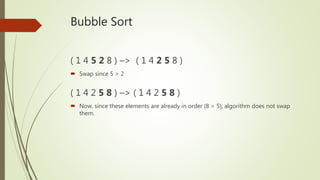
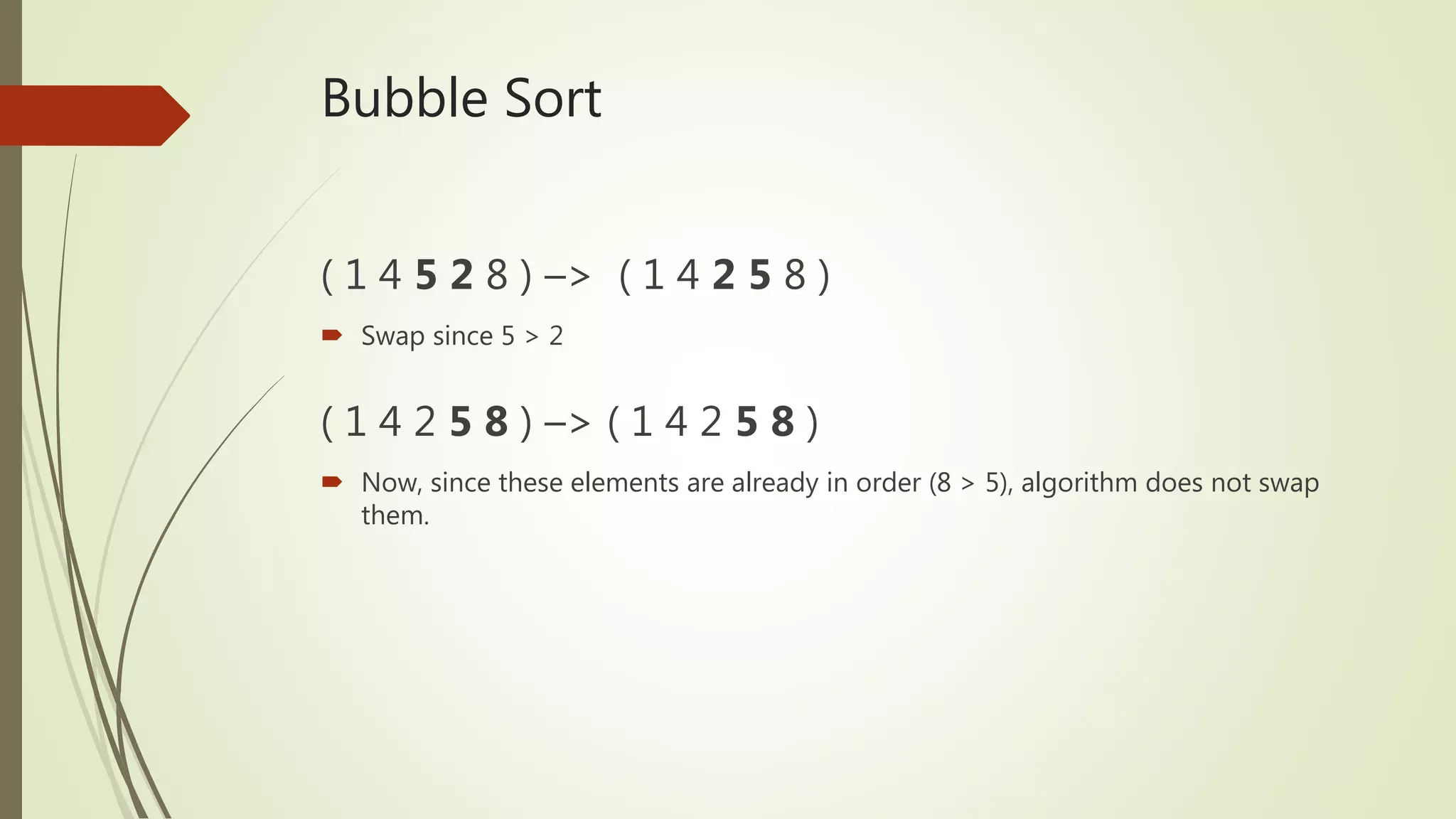
( 14 5 2 8 ) –> ( 1 4 2 5 8 )
Swap since 5 > 2
( 1 4 2 5 8 ) –> ( 1 4 2 5 8 )
Now, since these elements are already in order (8 > 5), algorithm does not swap
them.
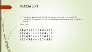
Bubble Sort
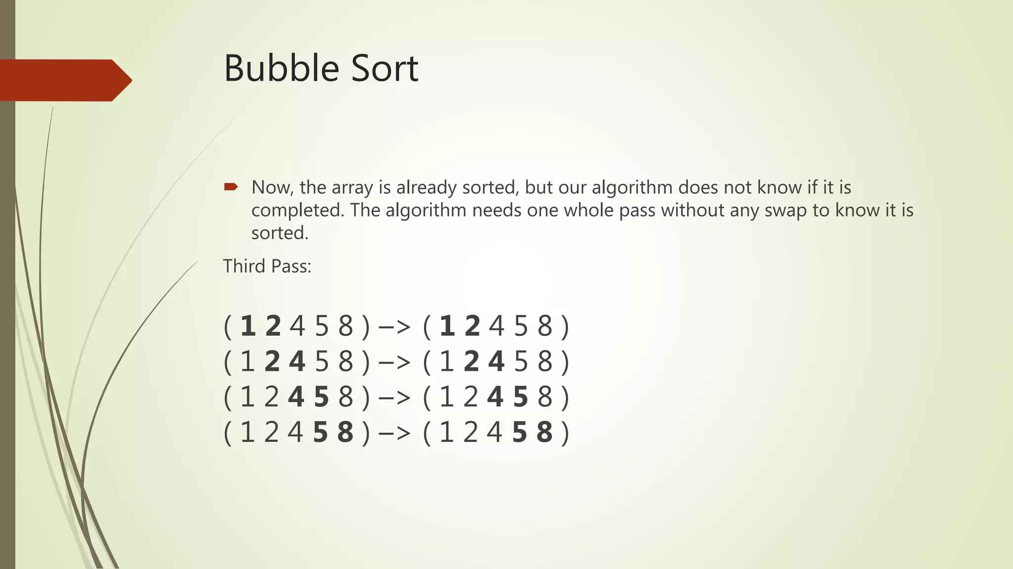
Now,the array is already sorted, but our algorithm does not know if it is
completed. The algorithm needs one whole pass without any swap to know it is
sorted.
Third Pass:
( 1 2 4 5 8 ) –> ( 1 2 4 5 8 )
( 1 2 4 5 8 ) –> ( 1 2 4 5 8 )
( 1 2 4 5 8 ) –> ( 1 2 4 5 8 )
( 1 2 4 5 8 ) –> ( 1 2 4 5 8 )
19.
Bubble Sort
Now,the array is already sorted, but our algorithm does not know if it is
completed. The algorithm needs one whole pass without any swap to know it is
sorted.
Third Pass:
( 1 2 4 5 8 ) –> ( 1 2 4 5 8 )
( 1 2 4 5 8 ) –> ( 1 2 4 5 8 )
( 1 2 4 5 8 ) –> ( 1 2 4 5 8 )
( 1 2 4 5 8 ) –> ( 1 2 4 5 8 )
20.
Bubble Sort
Advantages ofBubble sort:
Easy to understand.
Easy to implement.
In-place, no external memory is needed.
Performs greatly when the array is almost sorted.
21.
Bubble Sort
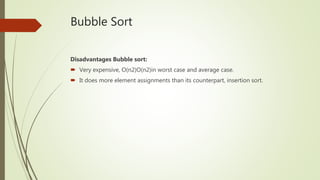
Disadvantages Bubblesort:
Very expensive, O(n2)O(n2)in worst case and average case.
It does more element assignments than its counterpart, insertion sort.


![Quick Sort
Here is how quicksort uses divide-and-conquer: think of sorting a sub
array[p…r], Where initially the sub array is array[0…n-1].
We take this set of array as an example:
40 20 10 80 60 50 7 30 100
0 1 2 3 4 5 6 7 8](https://image.slidesharecdn.com/presentation-171213023732/85/Analysis-of-Algorithm-Bubblesort-and-Quicksort-3-320.jpg)
![Quick Sort
Divide
1. Choose any element in the sub array [p…r] call this element Pivot.
We now have our Pivot which is 40 at array 0
40 20 10 80 60 50 7 30 100
0 1 2 3 4 5 6 7 8](https://image.slidesharecdn.com/presentation-171213023732/85/Analysis-of-Algorithm-Bubblesort-and-Quicksort-4-320.jpg)
![Quick Sort
Given again the array
40 20 10 80 60 50 7 30 100
0 1 2 3 4 5 6 7 8
7 20 10 30 40 50 80 60 100
<= Data [pivot] > Data [pivot]](https://image.slidesharecdn.com/presentation-171213023732/85/Analysis-of-Algorithm-Bubblesort-and-Quicksort-6-320.jpg)
![Quick Sort
Conquer
After dividing recursively sort each sub array
<= Data [pivot]
7 20 10 30
7 20 10 30
7 20 10 30
7 10 20 30
7 20 10 30
7 10 20 30
7 10 20 30](https://image.slidesharecdn.com/presentation-171213023732/85/Analysis-of-Algorithm-Bubblesort-and-Quicksort-7-320.jpg)
![Quick Sort
Conquer
After dividing recursively sort each sub array
> Data [pivot]
50 60 80 100
50 80 60 100
50 80 60 100
50 80 60 100
50 60 80 100
50 80 60 100
50 60 80 100
50 60 80 100](https://image.slidesharecdn.com/presentation-171213023732/85/Analysis-of-Algorithm-Bubblesort-and-Quicksort-8-320.jpg)


![Quick Sort
Here is how quicksort uses divide-and-conquer: think of sorting a sub
array[p…r], Where initially the sub array is array[0…n-1].
We take this set of array as an example:
40 20 10 80 60 50 7 30 100
0 1 2 3 4 5 6 7 8](https://image.slidesharecdn.com/presentation-171213023732/75/Analysis-of-Algorithm-Bubblesort-and-Quicksort-3-2048.jpg)
![Quick Sort
Divide
1. Choose any element in the sub array [p…r] call this element Pivot.
We now have our Pivot which is 40 at array 0
40 20 10 80 60 50 7 30 100
0 1 2 3 4 5 6 7 8](https://image.slidesharecdn.com/presentation-171213023732/75/Analysis-of-Algorithm-Bubblesort-and-Quicksort-4-2048.jpg)
![Quick Sort
Given again the array
40 20 10 80 60 50 7 30 100
0 1 2 3 4 5 6 7 8
7 20 10 30 40 50 80 60 100
<= Data [pivot] > Data [pivot]](https://image.slidesharecdn.com/presentation-171213023732/75/Analysis-of-Algorithm-Bubblesort-and-Quicksort-6-2048.jpg)
![Quick Sort
Conquer
After dividing recursively sort each sub array
<= Data [pivot]
7 20 10 30
7 20 10 30
7 20 10 30
7 10 20 30
7 20 10 30
7 10 20 30
7 10 20 30](https://image.slidesharecdn.com/presentation-171213023732/75/Analysis-of-Algorithm-Bubblesort-and-Quicksort-7-2048.jpg)
![Quick Sort
Conquer
After dividing recursively sort each sub array
> Data [pivot]
50 60 80 100
50 80 60 100
50 80 60 100
50 80 60 100
50 60 80 100
50 80 60 100
50 60 80 100
50 60 80 100](https://image.slidesharecdn.com/presentation-171213023732/75/Analysis-of-Algorithm-Bubblesort-and-Quicksort-8-2048.jpg)


![Data Structures - Lecture 8 [Sorting Algorithms]](https://cdn.slidesharecdn.com/ss_thumbnails/lecture-8sortingalgorithms-150205105023-conversion-gate02-thumbnail.jpg?width=600ounds&width=560&fit=bounds)


![UNIT V Searching Sorting Hashing Techniques [Autosaved].pptx](https://cdn.slidesharecdn.com/ss_thumbnails/unitvsearchingsortinghashingtechniquesautosaved-241126054304-95a69c51-thumbnail.jpg?width=600ounds&width=560&fit=bounds)
![UNIT V Searching Sorting Hashing Techniques [Autosaved].pptx](https://cdn.slidesharecdn.com/ss_thumbnails/unitvsearchingsortinghashingtechniquesautosaved-241014040608-74caa0f6-thumbnail.jpg?width=600ounds&width=560&fit=bounds)


