Download as PDF, PPTX
![ABOUT RESEARCH
Title
• “A General method applicable to the search for similarities
in the amino acid sequence of two proteins”
Authors
• Saul B. Needleman & Christian D. Wuncsch, Department of Biochemistry,
North-western University & Nuclear Medicine Service , V.A Research
Hospital ,Chicago, USA. (1969) [Cited by 8474]
S.B. Needleman & C.D. Wuncsch , “A General method applicable to the search for similarities in
the amino acid sequence of two proteins” , J. Mol . Biol .(1970) 48, 443- 453.](https://image.slidesharecdn.com/finalbipresentation2-140626013406-phpapp02/85/The-Needleman-Wunsch-Algorithm-for-Sequence-Alignment-2-320.jpg)


![ABOUT RESEARCH
Title
• “A General method applicable to the search for similarities
in the amino acid sequence of two proteins”
Authors
• Saul B. Needleman & Christian D. Wuncsch, Department of Biochemistry,
North-western University & Nuclear Medicine Service , V.A Research
Hospital ,Chicago, USA. (1969) [Cited by 8474]
S.B. Needleman & C.D. Wuncsch , “A General method applicable to the search for similarities in
the amino acid sequence of two proteins” , J. Mol . Biol .(1970) 48, 443- 453.](https://image.slidesharecdn.com/finalbipresentation2-140626013406-phpapp02/75/The-Needleman-Wunsch-Algorithm-for-Sequence-Alignment-2-2048.jpg)


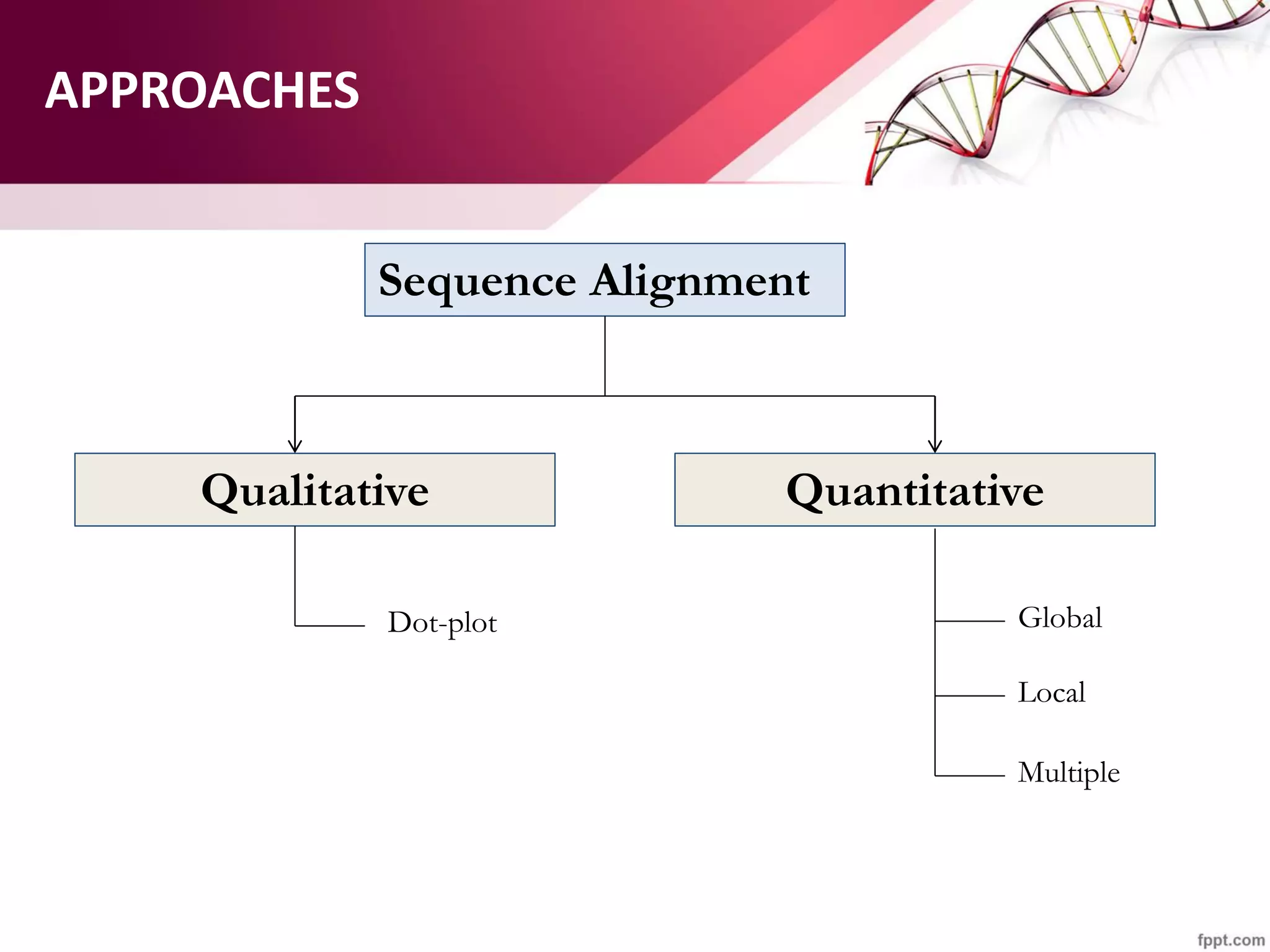
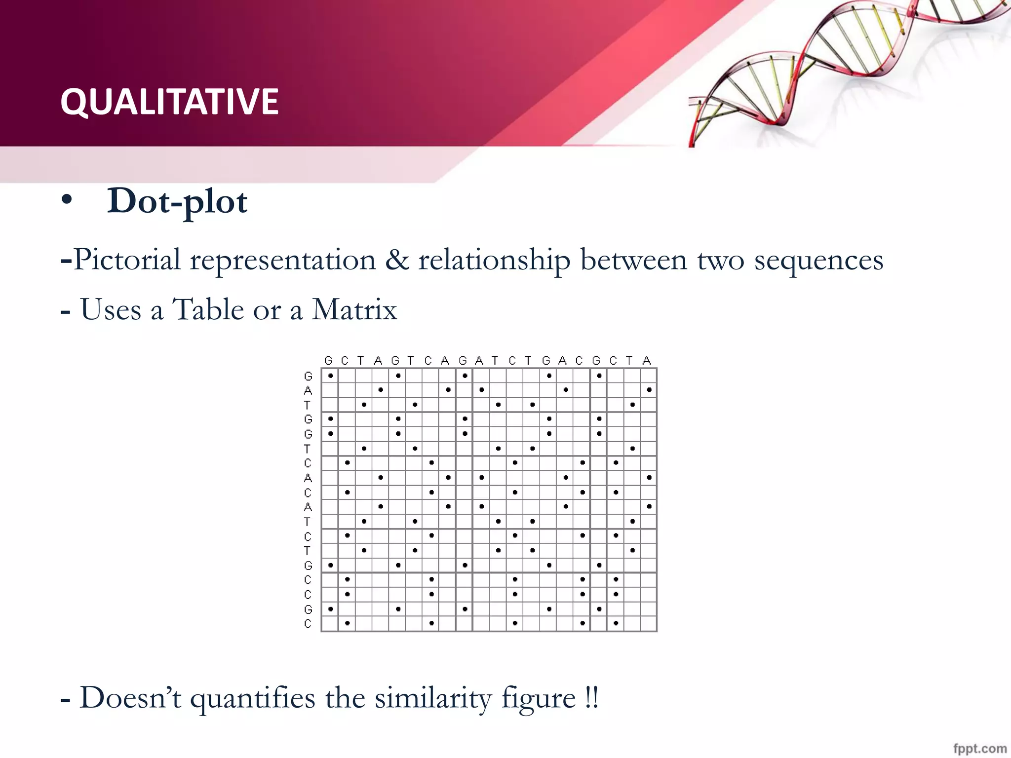
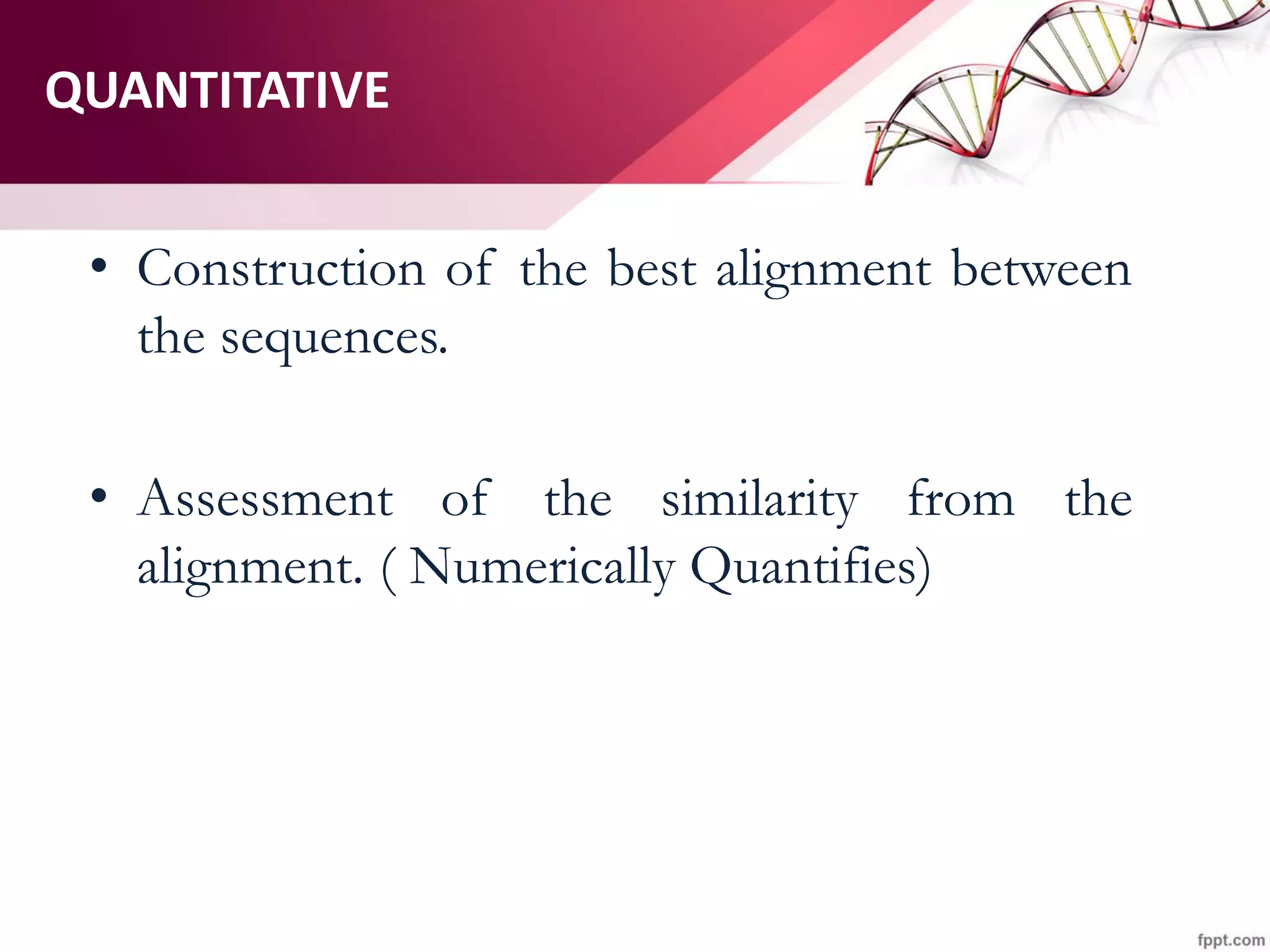
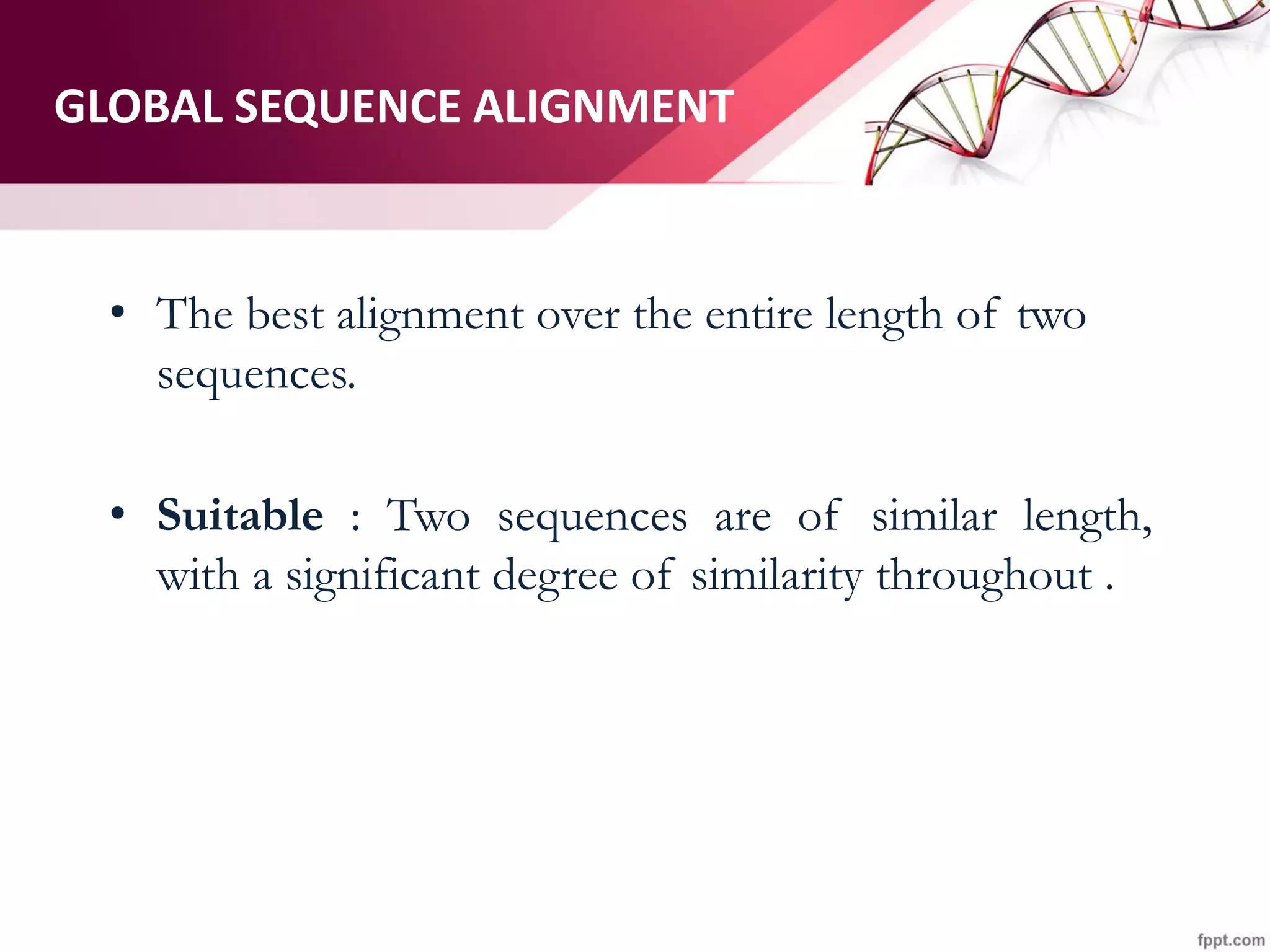

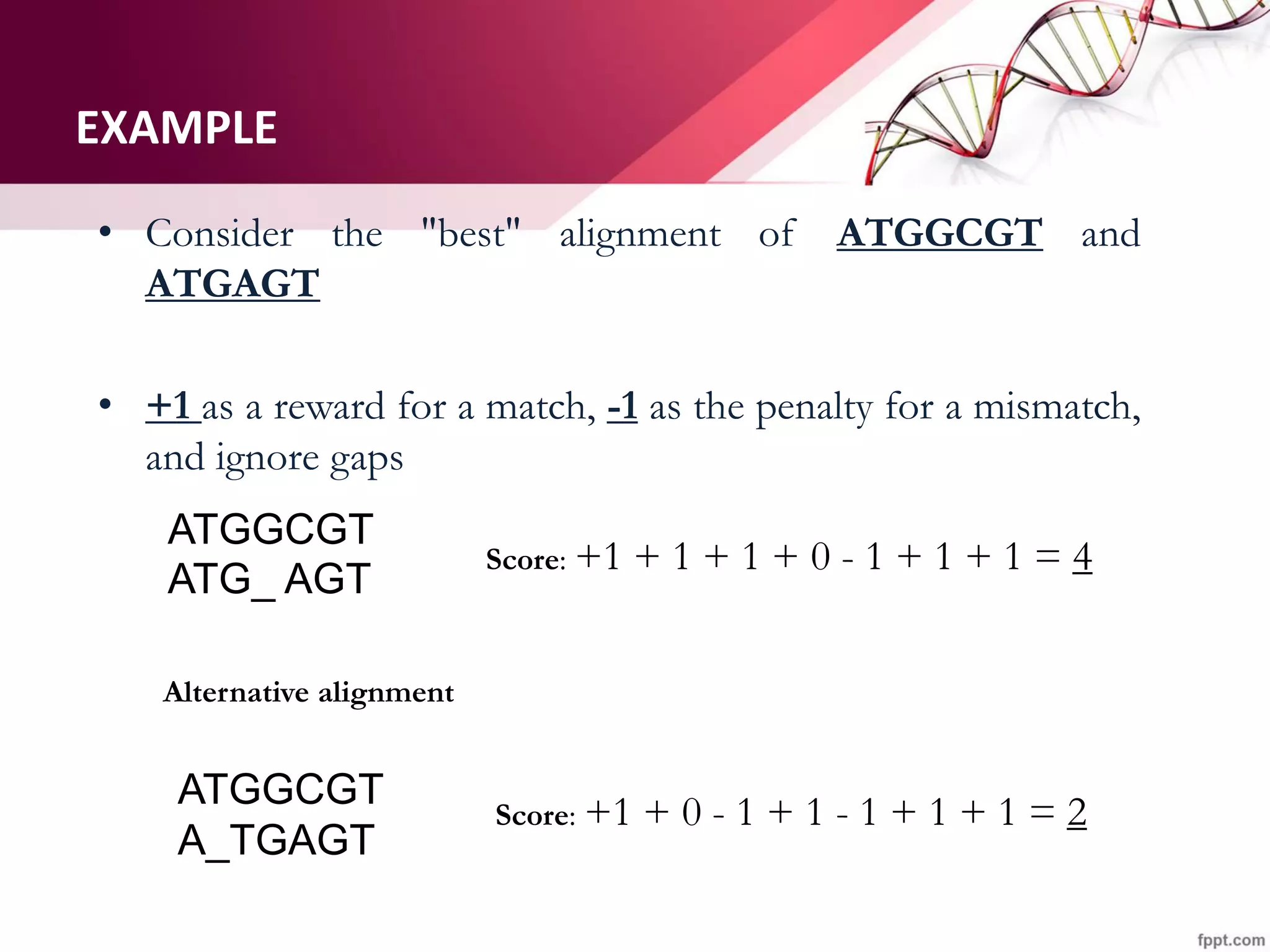


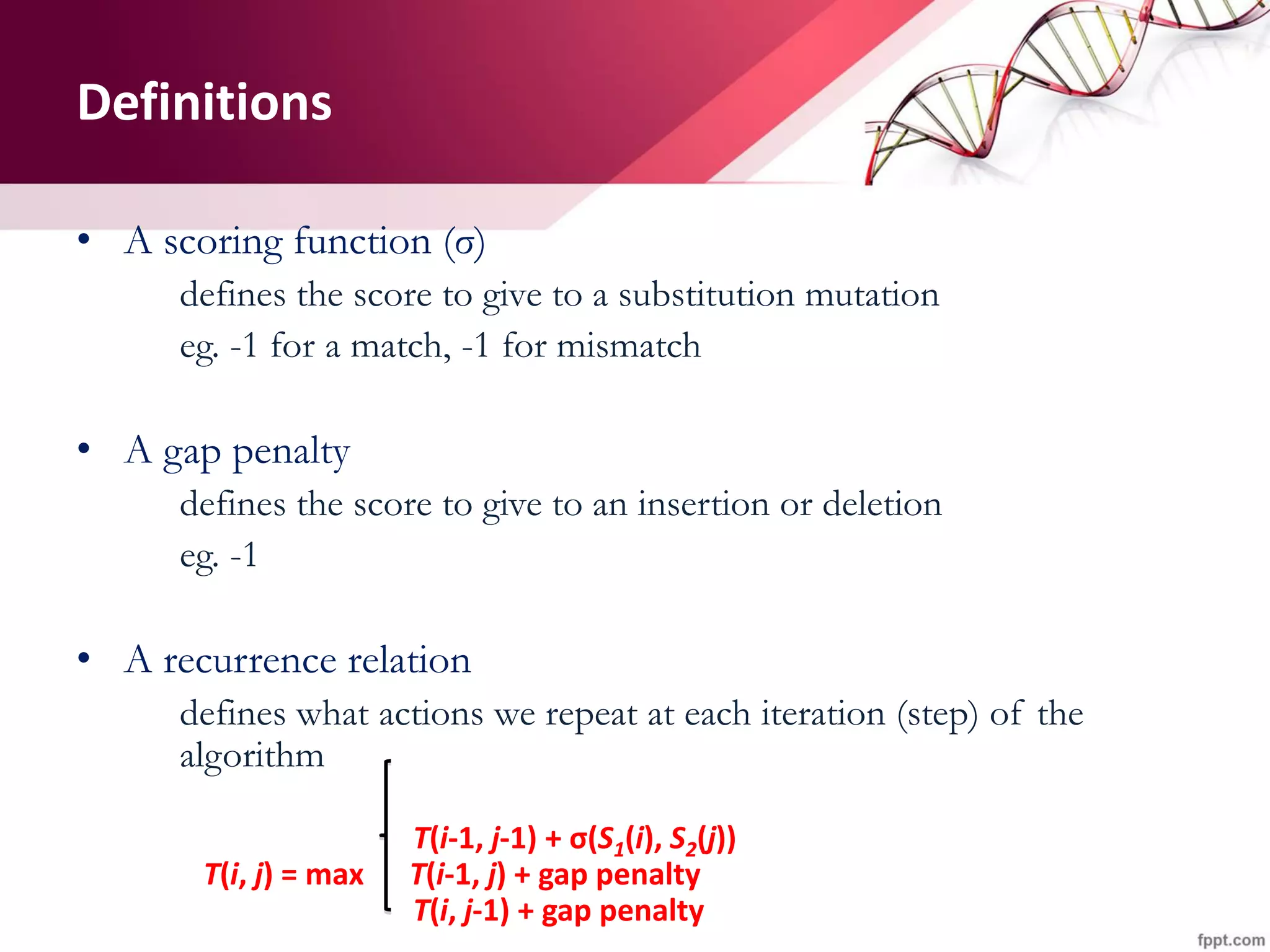
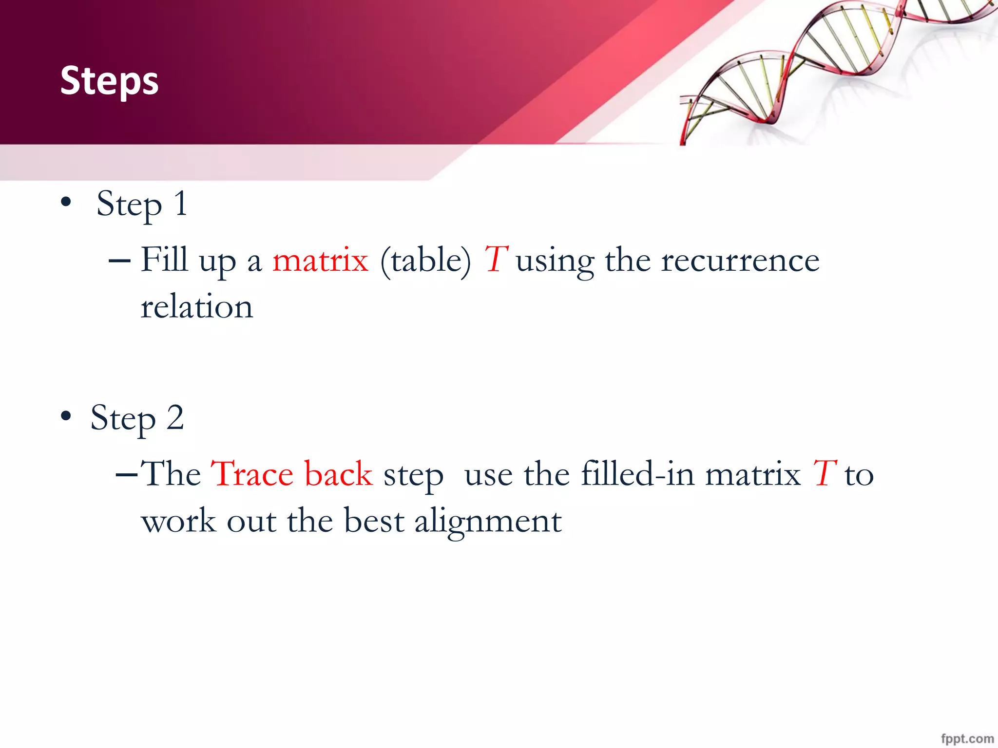

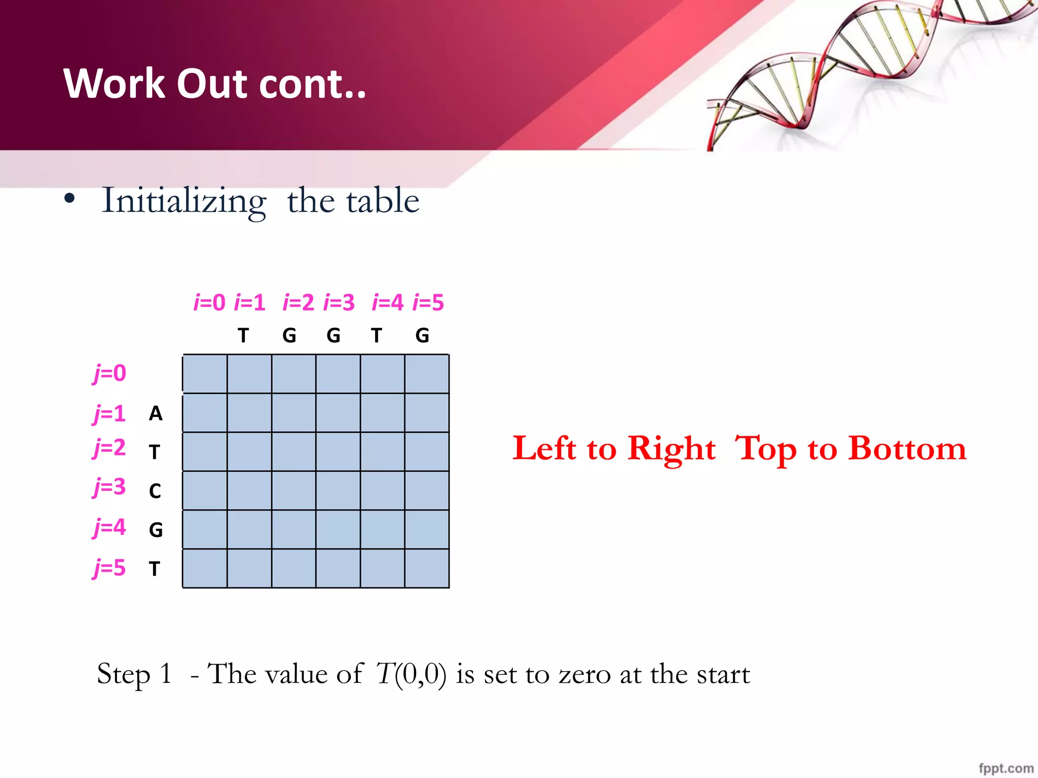
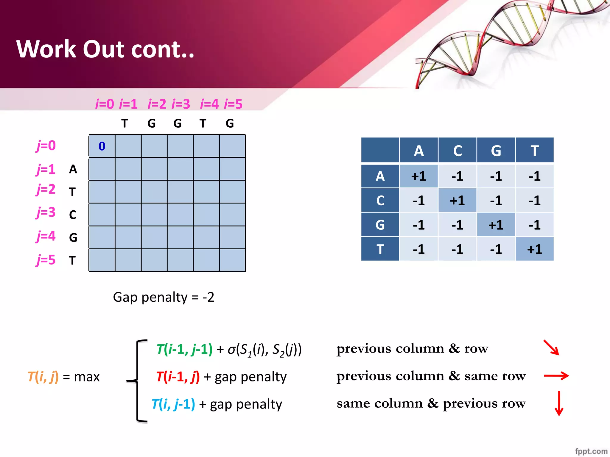
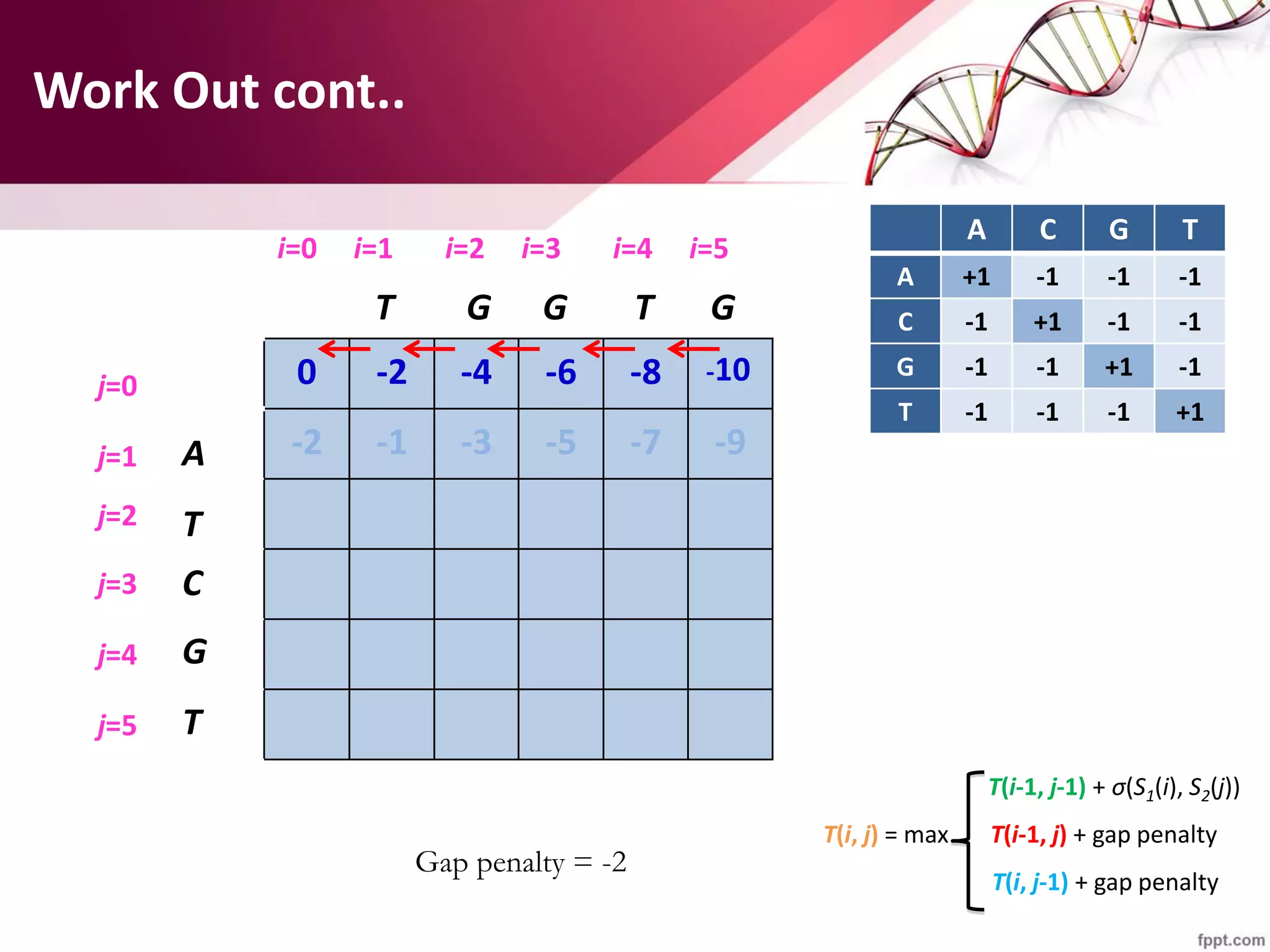

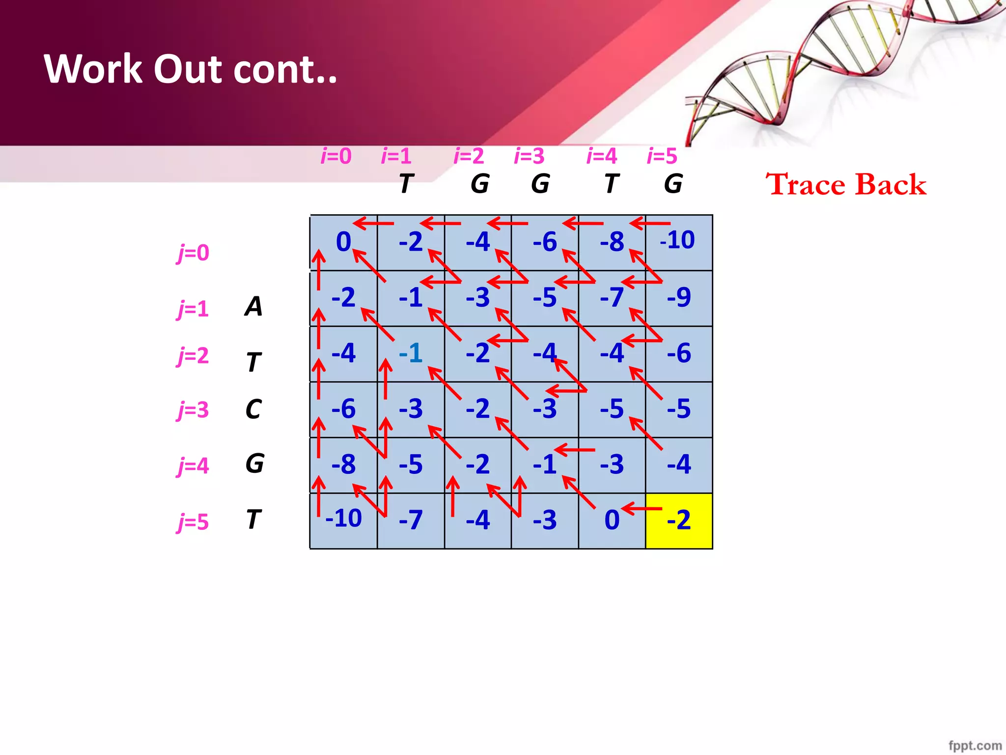
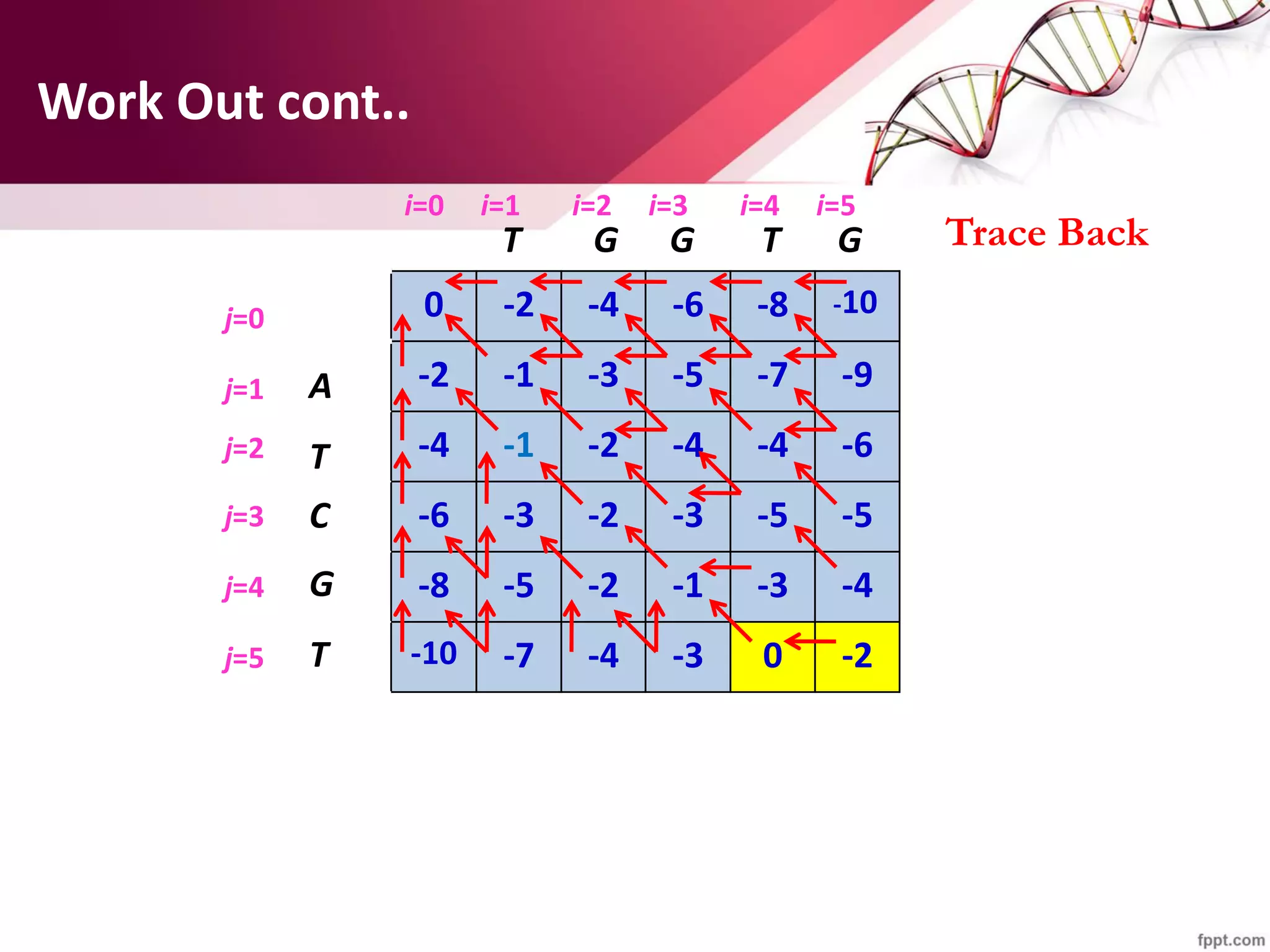
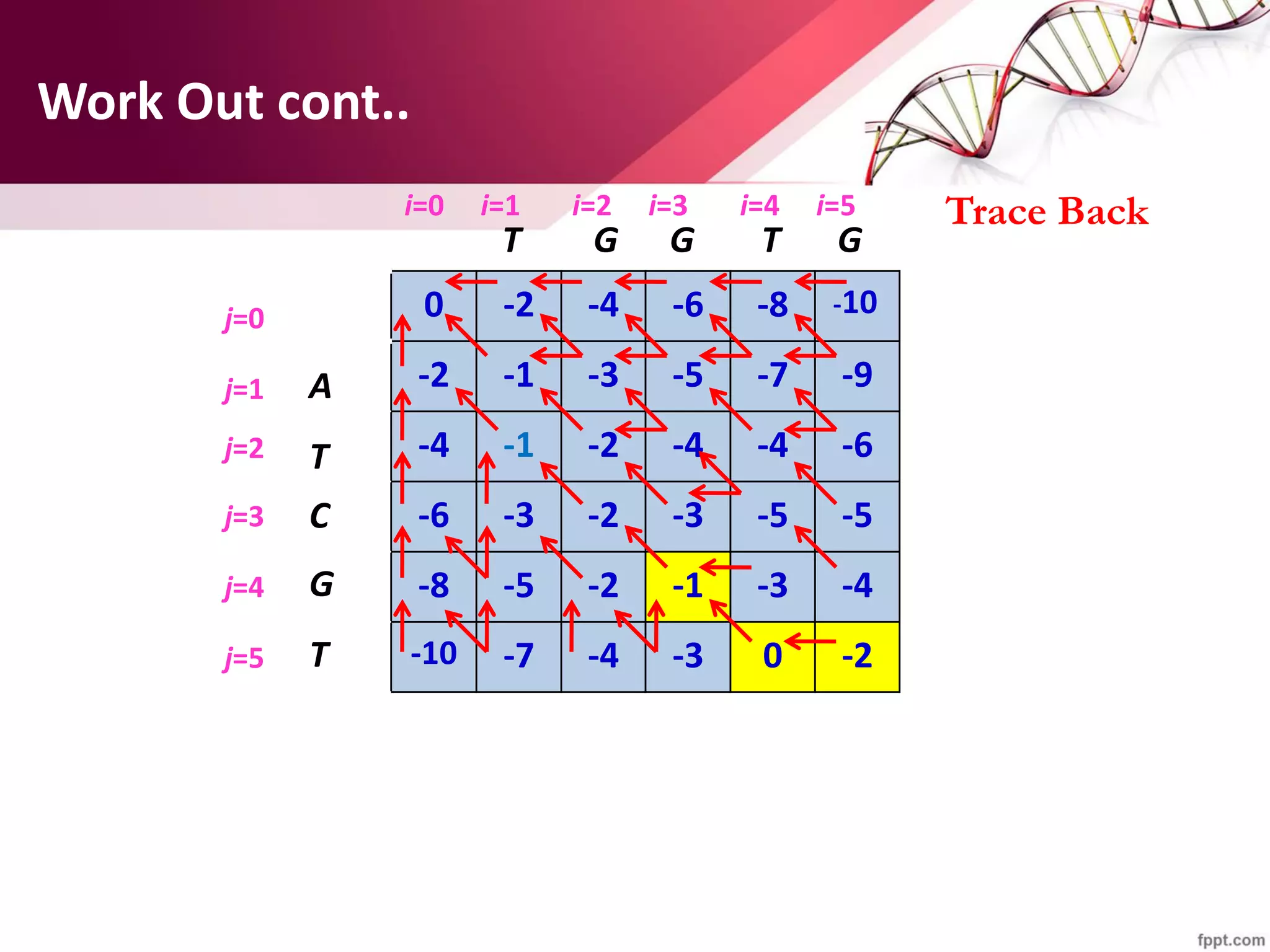
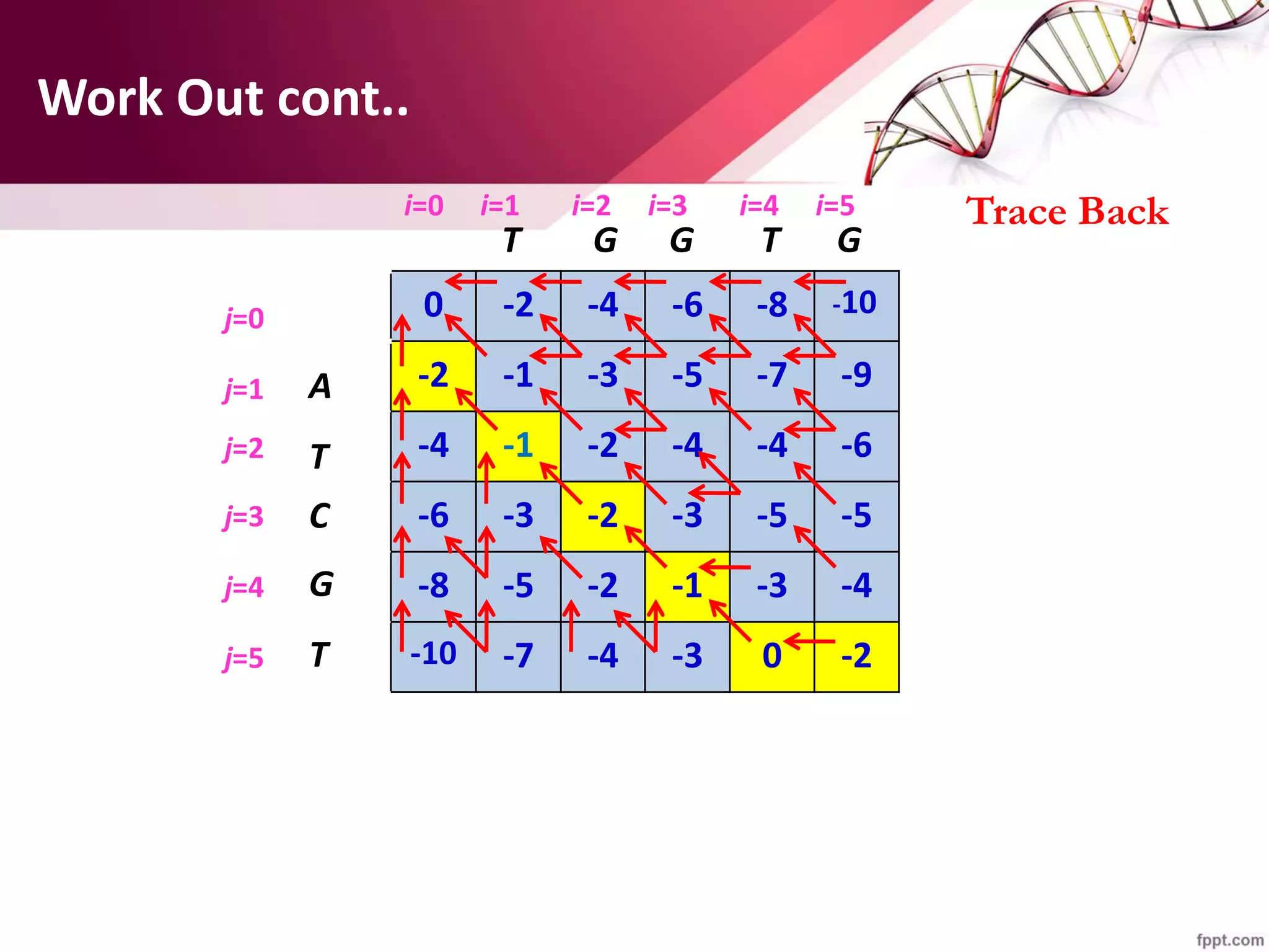
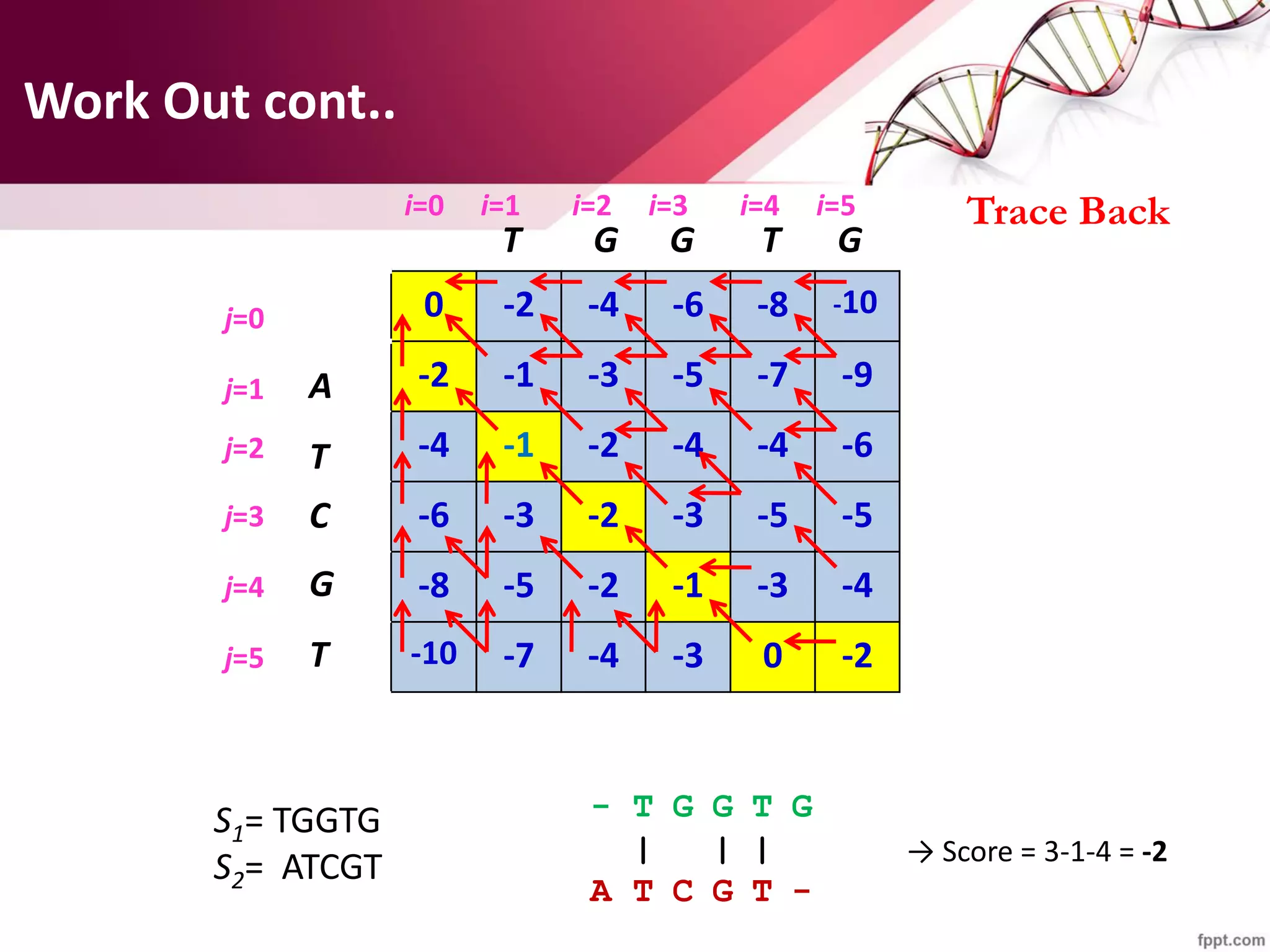
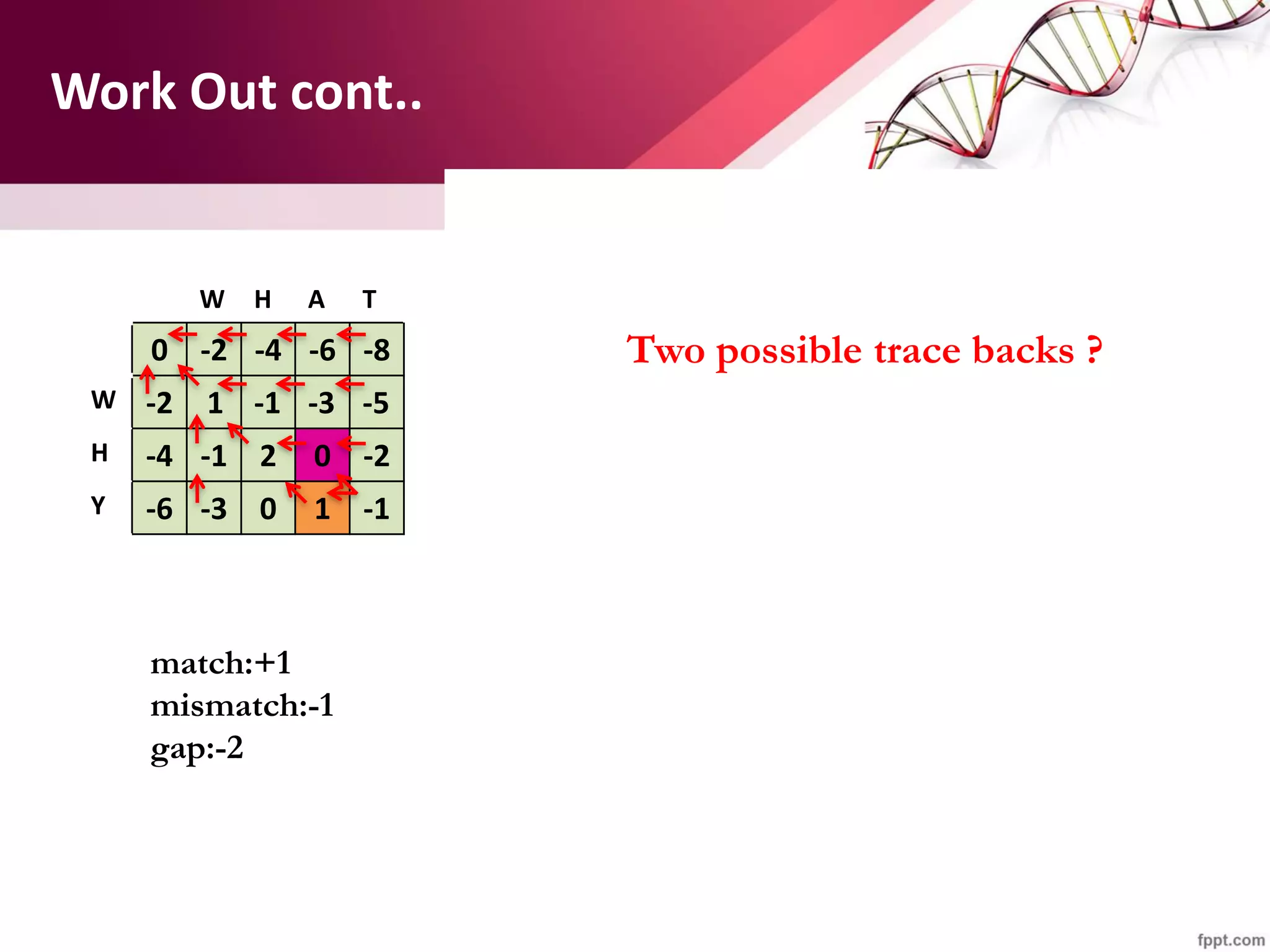


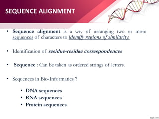
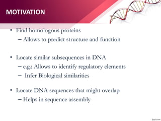
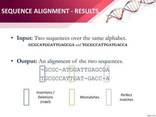
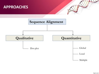
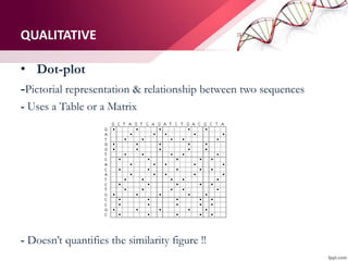
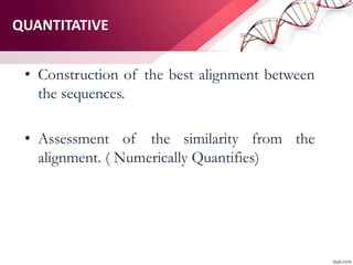
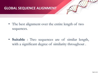
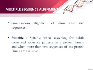
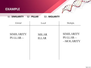
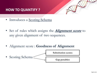
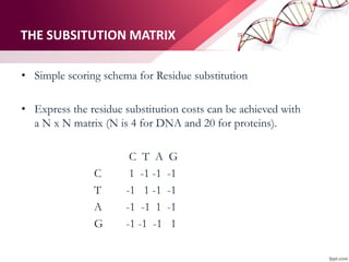
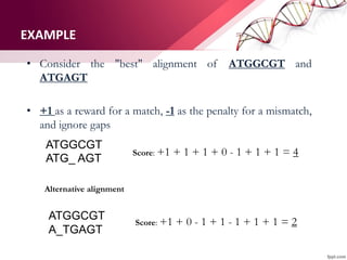
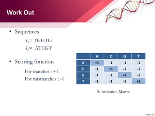
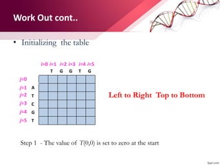
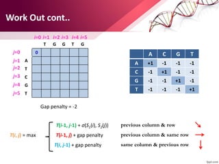
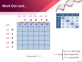
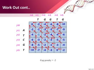
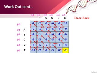
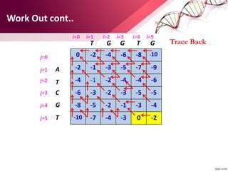
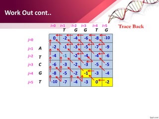
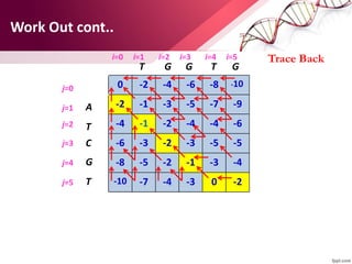
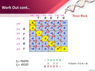
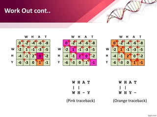
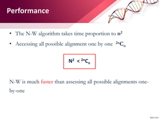
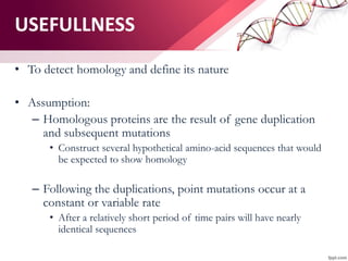
The document discusses the Needleman-Wunsch algorithm for global sequence alignment in bioinformatics, detailing its methodology and applications in comparing amino acid sequences of proteins. It outlines the fundamental components of sequence alignment, including scoring schemas, gap penalties, and the use of dynamic programming to efficiently solve alignment problems. This technique is crucial for predicting protein structure and function by identifying homologous sequences across different biological entities.


