Download as PDF, PPTX
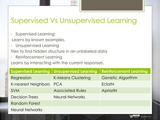


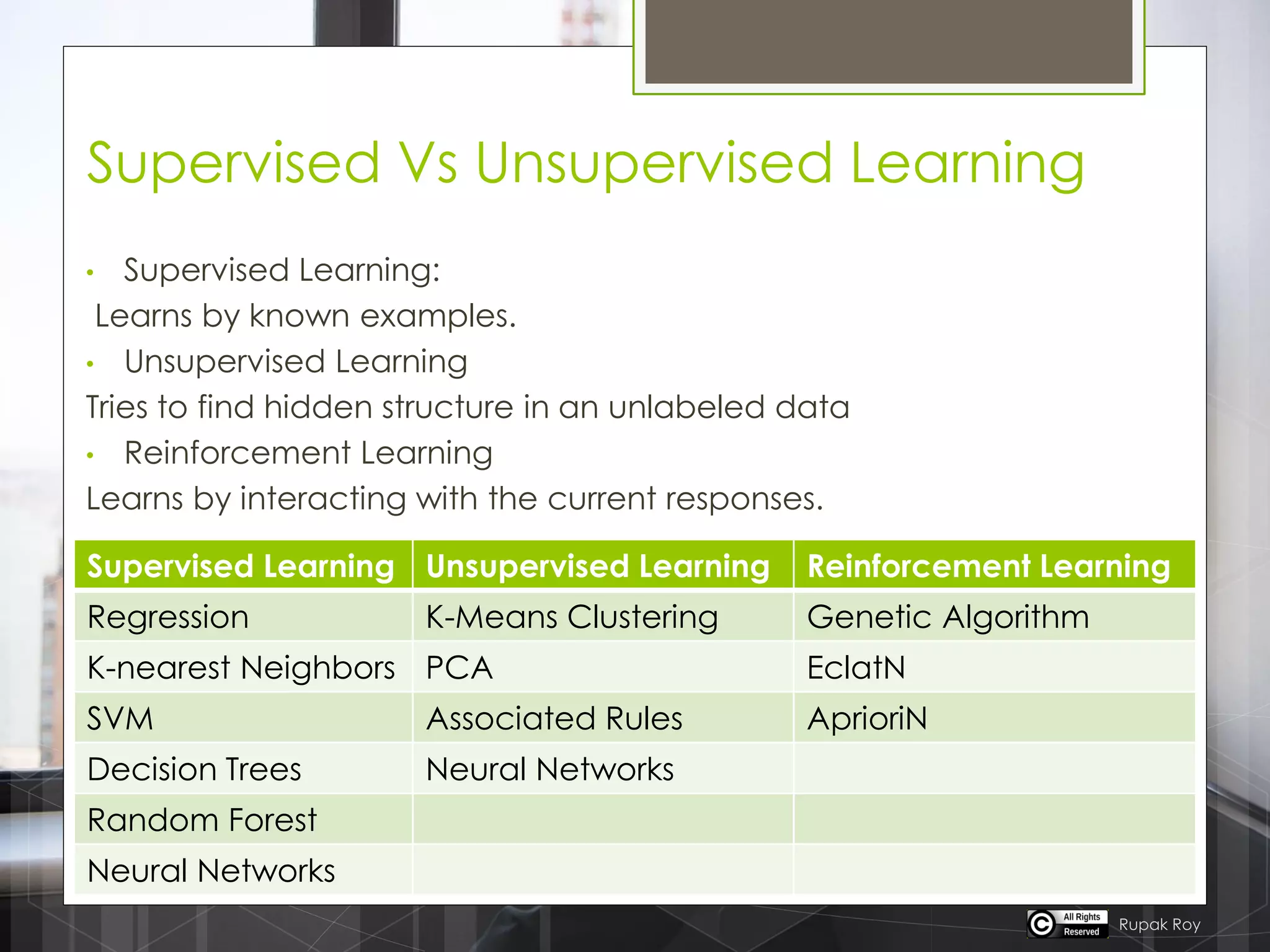
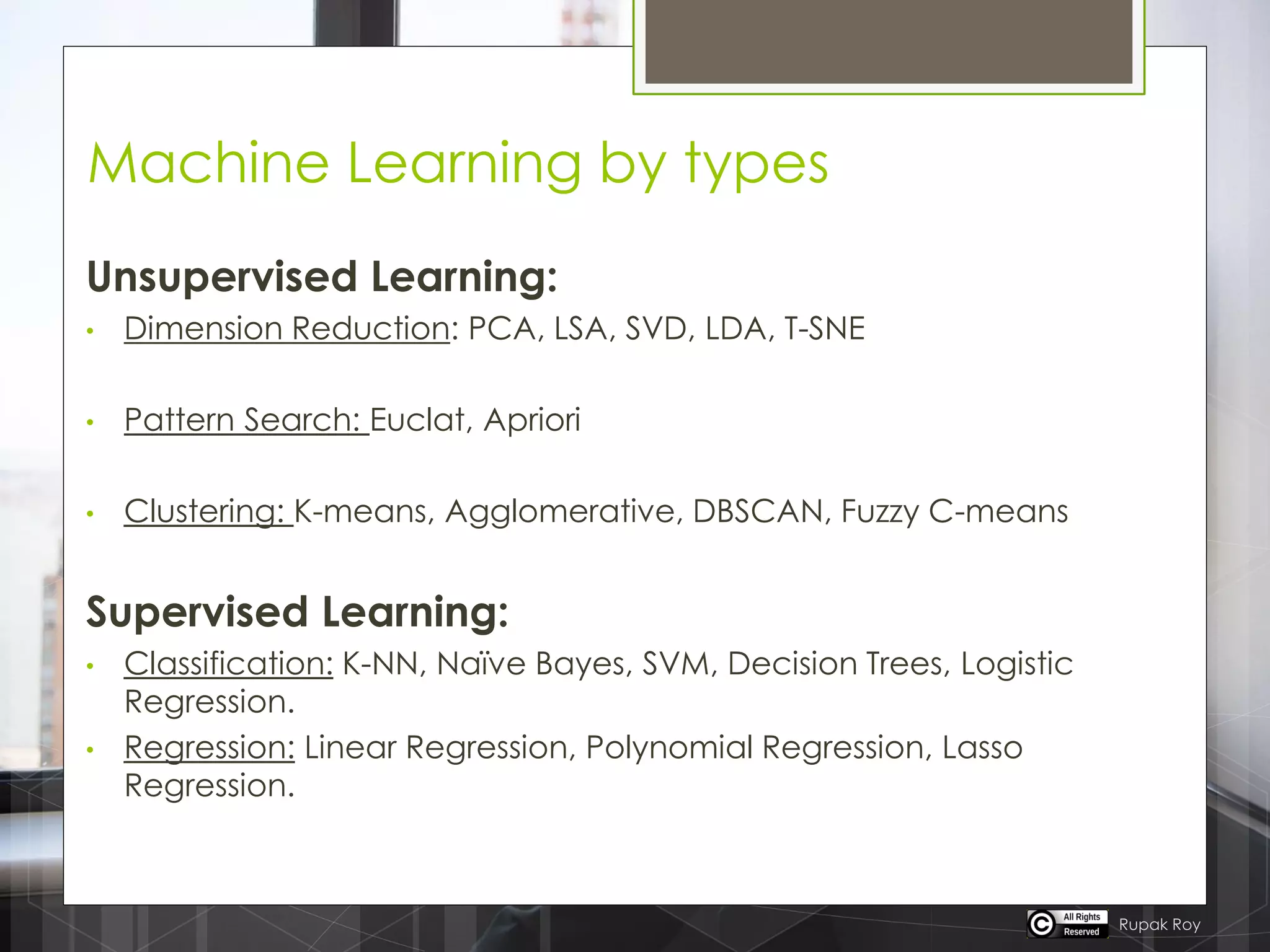
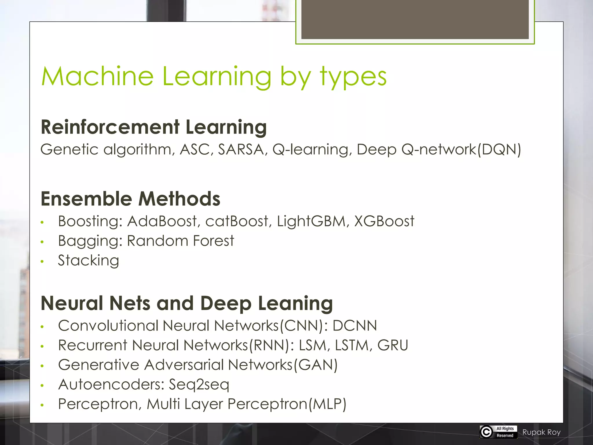

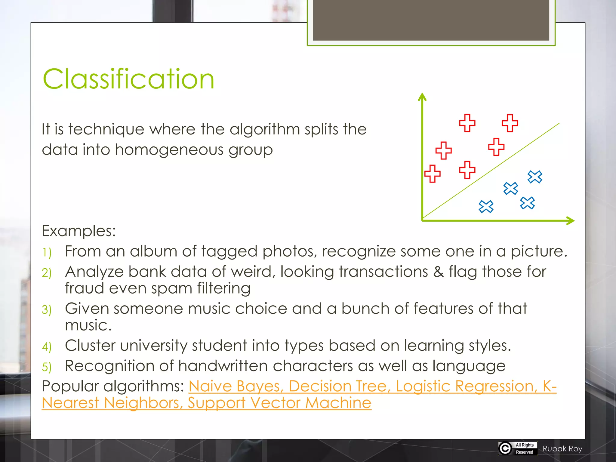
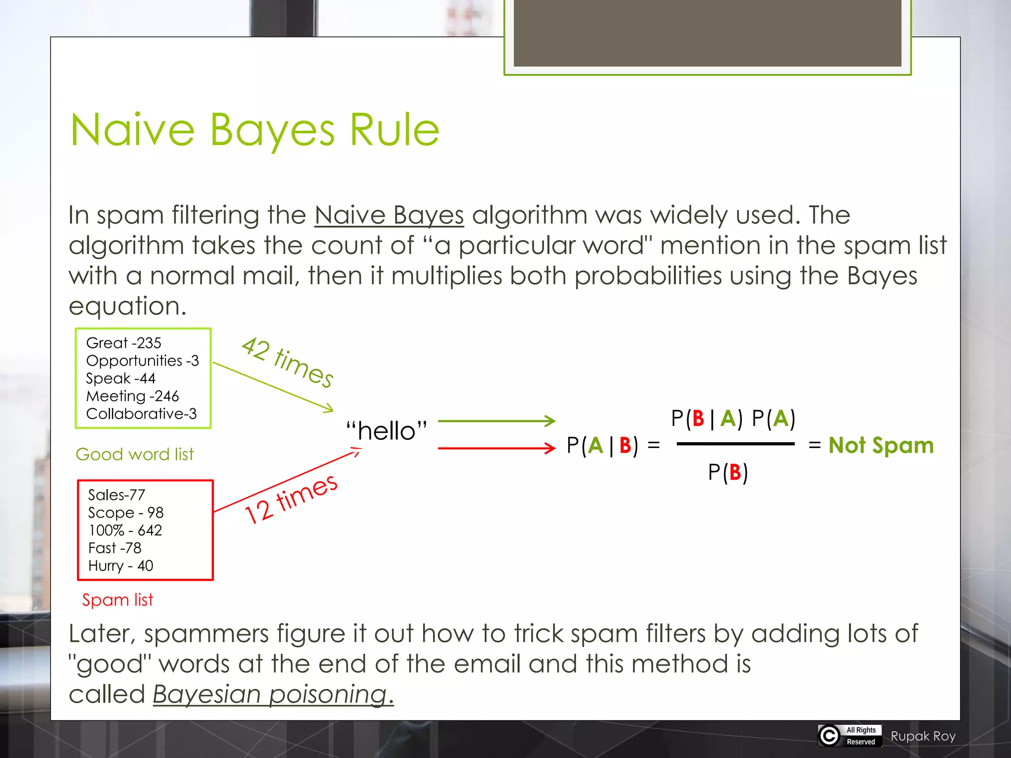

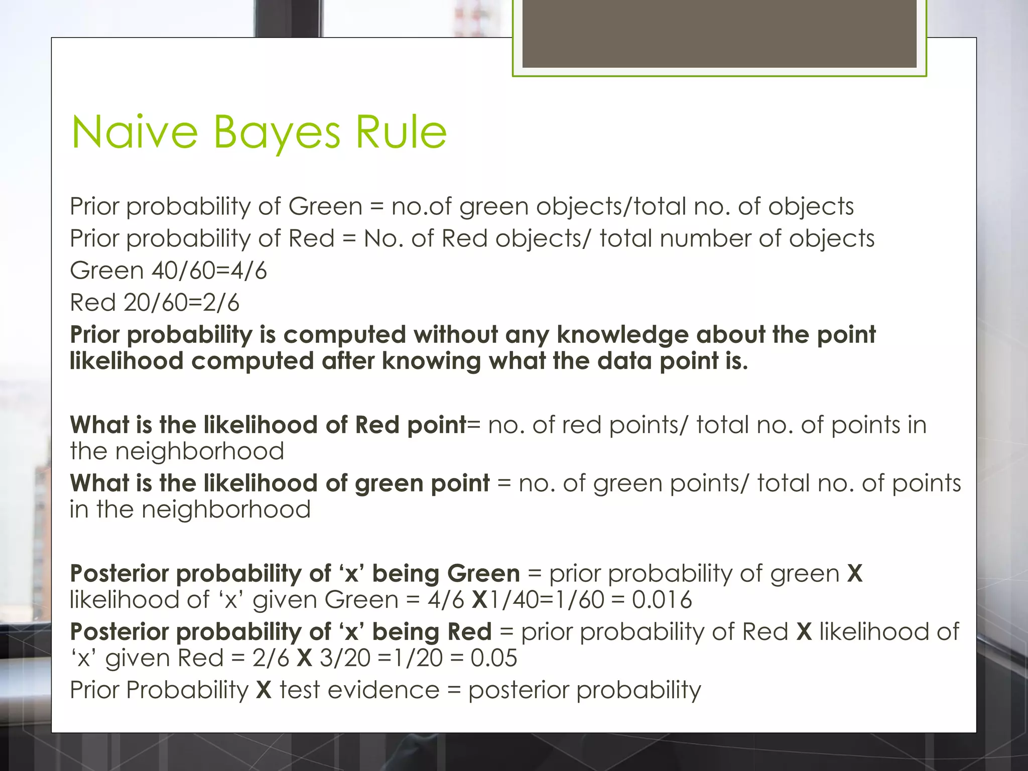


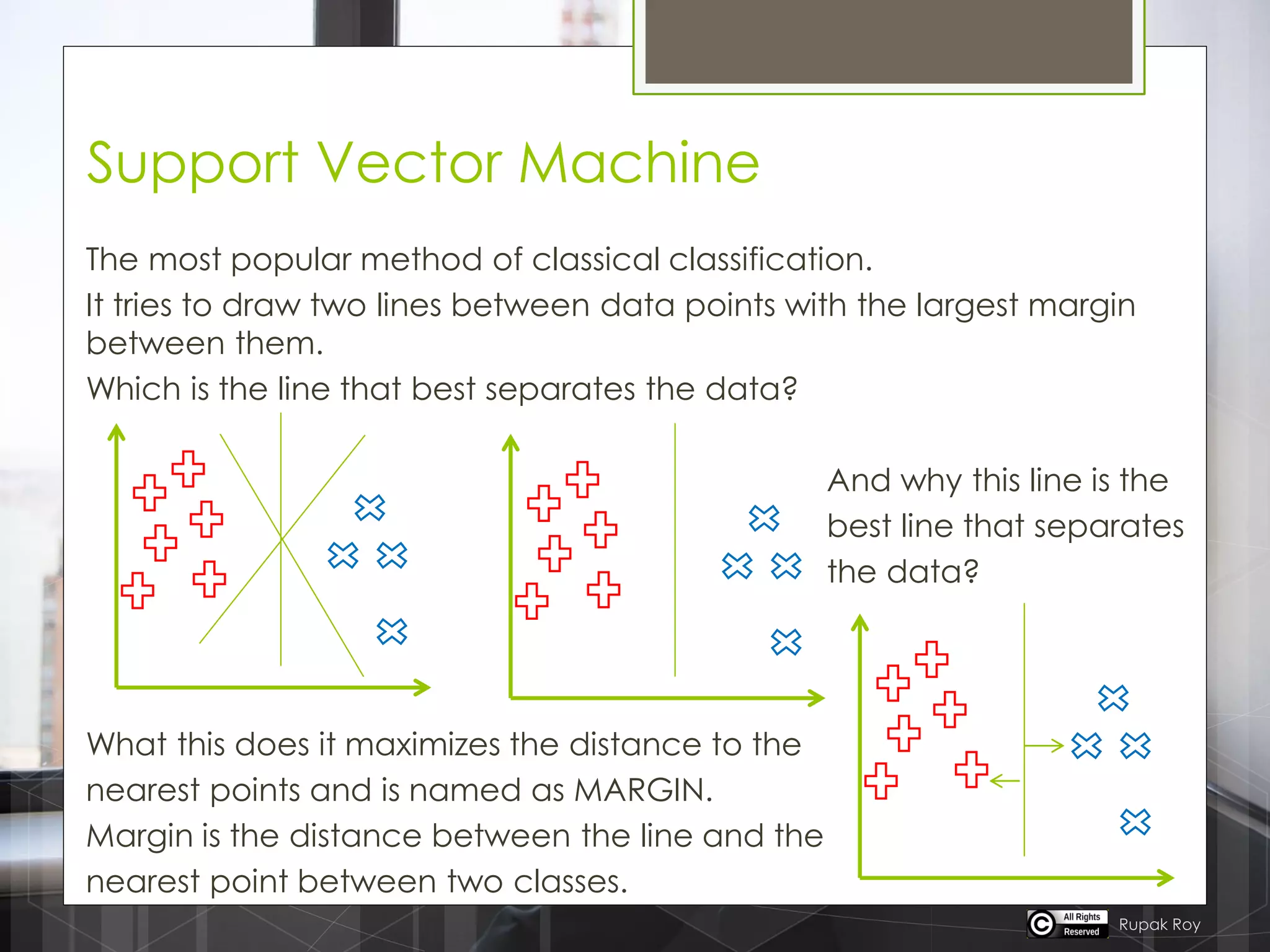

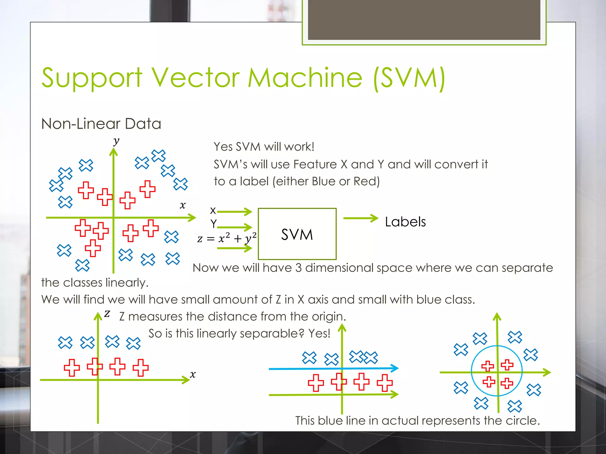
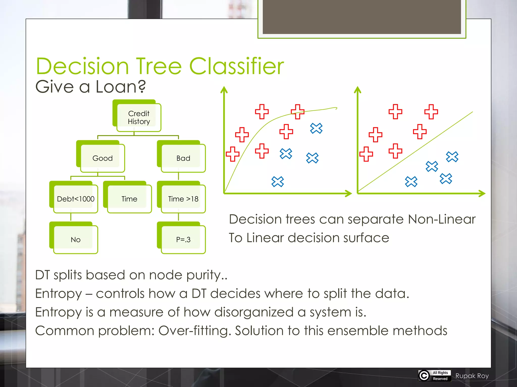

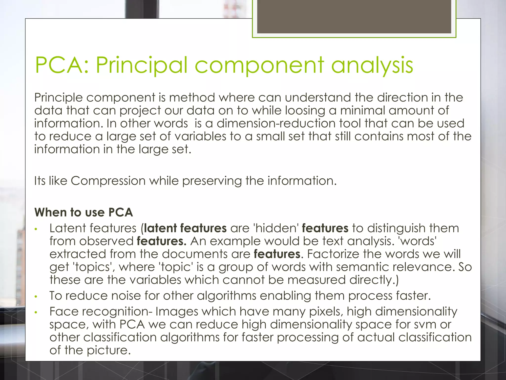

The document discusses various machine learning algorithms categorized into supervised, unsupervised, and reinforcement learning, explaining their unique mechanisms and applications. It notably details methods such as Naive Bayes, Support Vector Machines, and Decision Trees, alongside the importance of techniques like PCA for dimensionality reduction. Additionally, it addresses challenges like overfitting and the bias-variance trade-off in model training and performance.


![Matrix and determinant URT [Autosaved].pptx](https://cdn.slidesharecdn.com/ss_thumbnails/matrixanddeterminanturtautosaved-251018190340-9e6a6deb-thumbnail.jpg?width=600ounds&width=560&fit=bounds)


![RTP_AR_Basic_Learners' Workbook_KS2 [FOR REPRODUCTION] (1).pdf](https://cdn.slidesharecdn.com/ss_thumbnails/rtparbasiclearnersworkbookks2forreproduction1-251016024943-e51a16ac-thumbnail.jpg?width=600ounds&width=560&fit=bounds)

![Agentic Systems and Compliance - A brief intro [1.2]](https://cdn.slidesharecdn.com/ss_thumbnails/agenticsystemsandcompliace-1-251018025303-958a42ec-thumbnail.jpg?width=600ounds&width=560&fit=bounds)