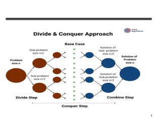
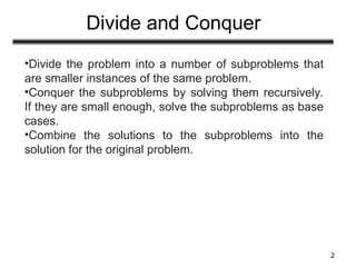
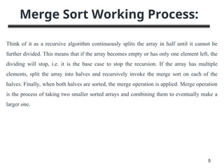
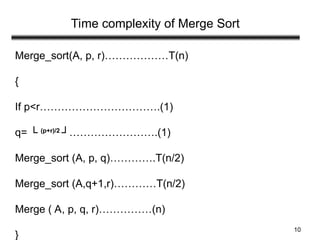
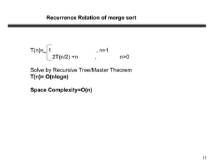
The document outlines the divide and conquer algorithm technique, detailing its process and applications such as merge sort, quick sort, and heap sort. It provides explanations of their respective time complexities, space complexities, and algorithms, including pseudo-code for implementation. Additionally, it describes binary search, its algorithm, and time complexities comparing it to linear search.


![7
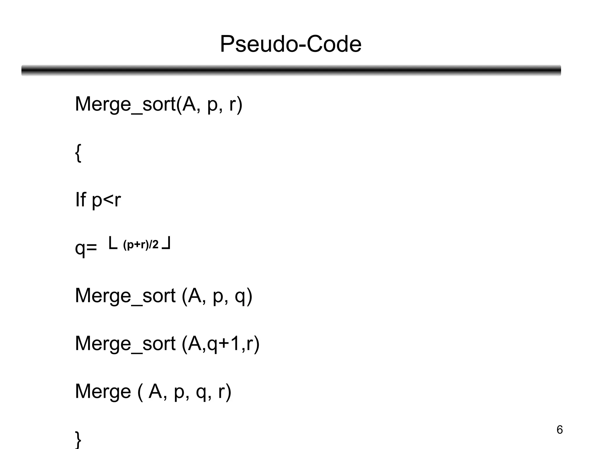
Pseudo-Code
Merge(A, p, q, r)
{
n1=q-p+1 //count the number of elements in first list
n2=r-q
Let L [ 1………..n1+1] and
R[1…….n2+1] be the two new arrays
For(i=1 to n1)
L[i]=A[p+i-1] // copy array into first list
For(j=1 to n2)
R[j]=A[q+j]
L[n1+1]=∞
R[n2+1]=∞](https://image.slidesharecdn.com/unit-2-sortingmergequickheapbinarysearach-240913172104-e5c4db68/85/Unit-2-Sorting-Merge-Quick-Heap-Binary-Searach-ppt-7-320.jpg)
![8
For(k=p to r) //k will be incremented at every step
If(L[i]<= R[j])
A[k]=L[i]
i+1
Else
A[k]=R[j]
j=j+1](https://image.slidesharecdn.com/unit-2-sortingmergequickheapbinarysearach-240913172104-e5c4db68/85/Unit-2-Sorting-Merge-Quick-Heap-Binary-Searach-ppt-8-320.jpg)

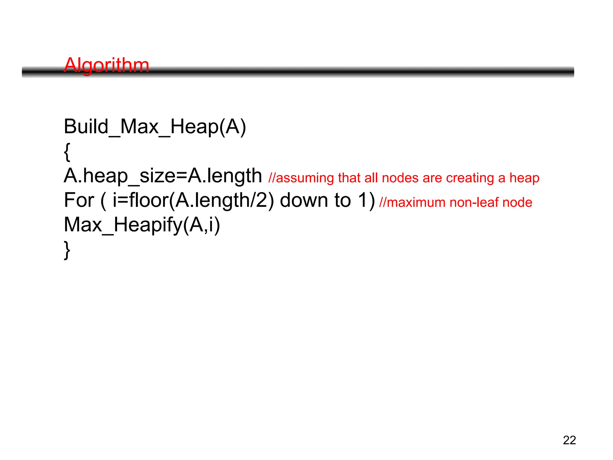
![21
Algorithm
Heap_sort(A)
{
Build_max_heap(A)
For i= length[A] down to 2
Do exchange A[1]=A[i]
Heap_size[A]=Heap_size[A-1]
Max_Heapify(A,1)
}](https://image.slidesharecdn.com/unit-2-sortingmergequickheapbinarysearach-240913172104-e5c4db68/85/Unit-2-Sorting-Merge-Quick-Heap-Binary-Searach-ppt-21-320.jpg)

![23
Max_heapify(A,i)
{
l =2i
r =2 i+1
If(l <=A.heapsize and A[l]>A[i]) //if leftchild exists & greater than parent
Largest=l
Else largest=i
If(r <=A.heapsize and A[r]>A[largest])
Largest=r
If(largest != i)
Exchange A[i] with A[largest]
Max_heapify(A,largest)
}](https://image.slidesharecdn.com/unit-2-sortingmergequickheapbinarysearach-240913172104-e5c4db68/85/Unit-2-Sorting-Merge-Quick-Heap-Binary-Searach-ppt-23-320.jpg)
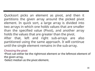
![31
Partition(A, p, r)
{
X=A[r]
i=p-1
For(j=p to r-1)
{
If(A[ j ]<=x)
{
i=i+1
Exchange A[i] with A[j]
}
}
Exchange A[i+1] with A[r]
Return (i+1)
}](https://image.slidesharecdn.com/unit-2-sortingmergequickheapbinarysearach-240913172104-e5c4db68/85/Unit-2-Sorting-Merge-Quick-Heap-Binary-Searach-ppt-31-320.jpg)

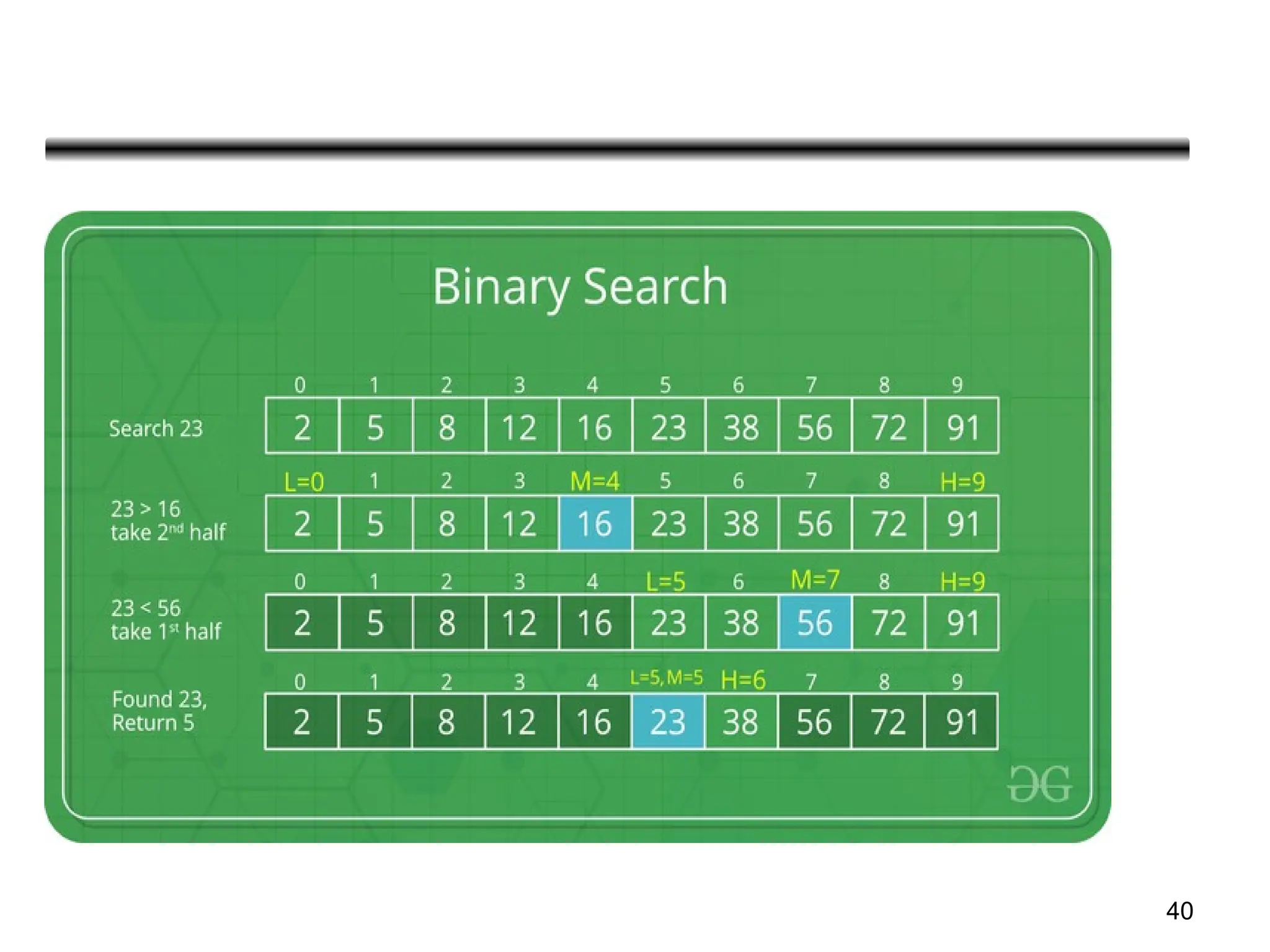
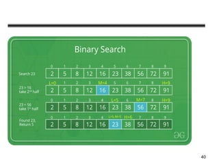
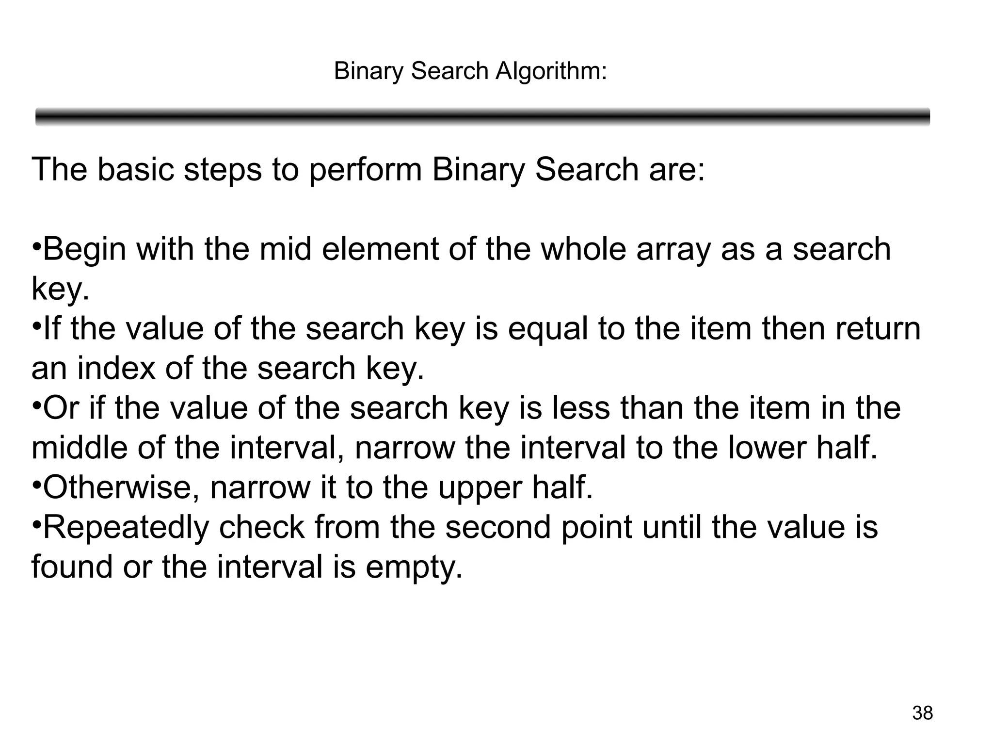
![39
binarySearch(arr, x, low, high)
repeat till low = high
mid = (low + high)/2
if (x == arr[mid])
return mid
else if (x > arr[mid]) // x is on the right side
low = mid + 1
else // x is on the left side
high = mid - 1
Binary Search Algorithm](https://image.slidesharecdn.com/unit-2-sortingmergequickheapbinarysearach-240913172104-e5c4db68/85/Unit-2-Sorting-Merge-Quick-Heap-Binary-Searach-ppt-39-320.jpg)


![7
Pseudo-Code
Merge(A, p, q, r)
{
n1=q-p+1 //count the number of elements in first list
n2=r-q
Let L [ 1………..n1+1] and
R[1…….n2+1] be the two new arrays
For(i=1 to n1)
L[i]=A[p+i-1] // copy array into first list
For(j=1 to n2)
R[j]=A[q+j]
L[n1+1]=∞
R[n2+1]=∞](https://image.slidesharecdn.com/unit-2-sortingmergequickheapbinarysearach-240913172104-e5c4db68/75/Unit-2-Sorting-Merge-Quick-Heap-Binary-Searach-ppt-7-2048.jpg)
![8
For(k=p to r) //k will be incremented at every step
If(L[i]<= R[j])
A[k]=L[i]
i+1
Else
A[k]=R[j]
j=j+1](https://image.slidesharecdn.com/unit-2-sortingmergequickheapbinarysearach-240913172104-e5c4db68/75/Unit-2-Sorting-Merge-Quick-Heap-Binary-Searach-ppt-8-2048.jpg)


![21
Algorithm
Heap_sort(A)
{
Build_max_heap(A)
For i= length[A] down to 2
Do exchange A[1]=A[i]
Heap_size[A]=Heap_size[A-1]
Max_Heapify(A,1)
}](https://image.slidesharecdn.com/unit-2-sortingmergequickheapbinarysearach-240913172104-e5c4db68/75/Unit-2-Sorting-Merge-Quick-Heap-Binary-Searach-ppt-21-2048.jpg)
![23
Max_heapify(A,i)
{
l =2i
r =2 i+1
If(l <=A.heapsize and A[l]>A[i]) //if leftchild exists & greater than parent
Largest=l
Else largest=i
If(r <=A.heapsize and A[r]>A[largest])
Largest=r
If(largest != i)
Exchange A[i] with A[largest]
Max_heapify(A,largest)
}](https://image.slidesharecdn.com/unit-2-sortingmergequickheapbinarysearach-240913172104-e5c4db68/75/Unit-2-Sorting-Merge-Quick-Heap-Binary-Searach-ppt-23-2048.jpg)

![31
Partition(A, p, r)
{
X=A[r]
i=p-1
For(j=p to r-1)
{
If(A[ j ]<=x)
{
i=i+1
Exchange A[i] with A[j]
}
}
Exchange A[i+1] with A[r]
Return (i+1)
}](https://image.slidesharecdn.com/unit-2-sortingmergequickheapbinarysearach-240913172104-e5c4db68/75/Unit-2-Sorting-Merge-Quick-Heap-Binary-Searach-ppt-31-2048.jpg)


![39
binarySearch(arr, x, low, high)
repeat till low = high
mid = (low + high)/2
if (x == arr[mid])
return mid
else if (x > arr[mid]) // x is on the right side
low = mid + 1
else // x is on the left side
high = mid - 1
Binary Search Algorithm](https://image.slidesharecdn.com/unit-2-sortingmergequickheapbinarysearach-240913172104-e5c4db68/75/Unit-2-Sorting-Merge-Quick-Heap-Binary-Searach-ppt-39-2048.jpg)