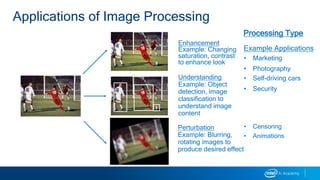
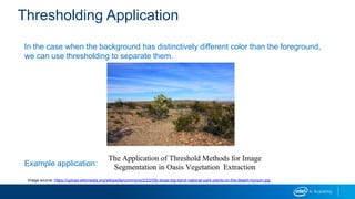
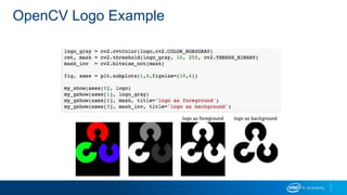
This document provides a 3-sentence summary of a legal notice and disclaimer document:
The document states that any Intel technologies discussed are for informational purposes only and Intel makes no warranties regarding the information. It notes that performance may vary depending on system configuration and that source code samples are released under an Intel license agreement. The document also provides legal notices and disclaimers regarding Intel trademarks and copyright.


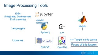

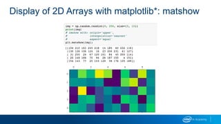
![Imshow arguments
o (m,n):
Rows, columns: NOT x,y coordinates
Can (m,n,3) and (m,n,4)
Values uint8 or float in [0,1]
(m,n,3) = RGB
(m,n,4) = RGBA
A alpha
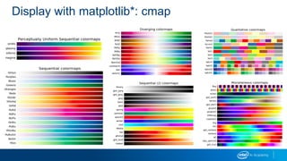
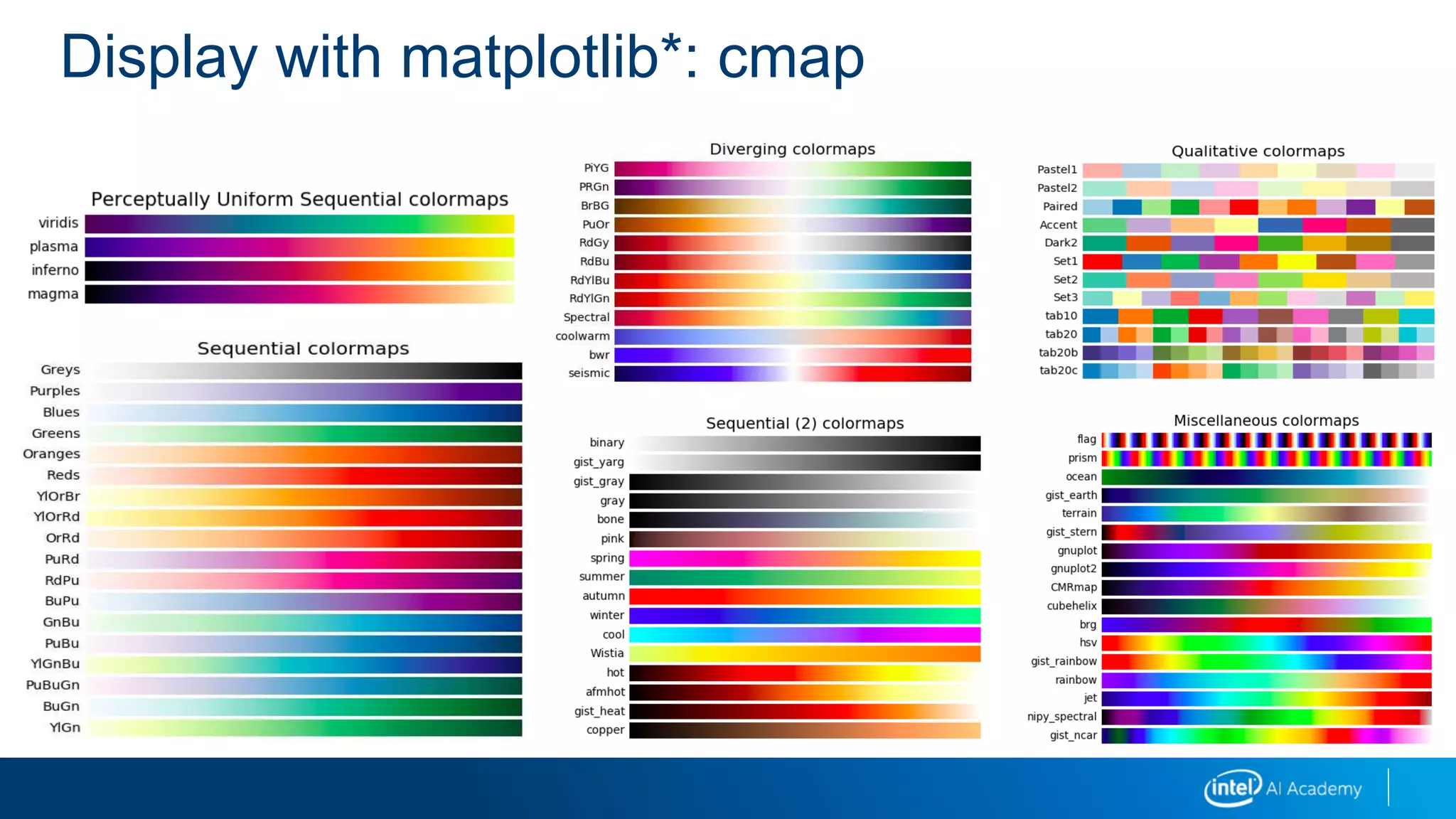
o “cmap”
Color map: can be RGB, grayscale, and so on
See upcoming slide for examples
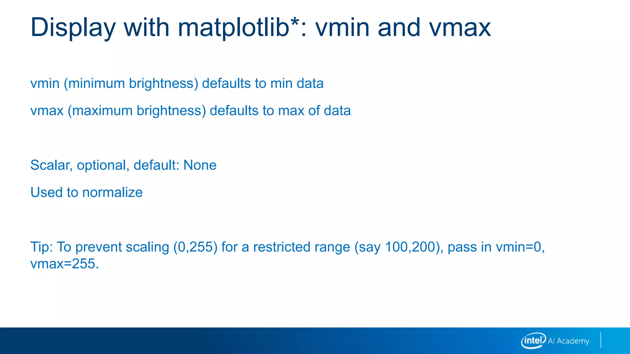
o “vmin”, “vmax”
Used to change brightness
Display with matplotlib*: imshow](https://image.slidesharecdn.com/02imageprocessing-190218095646/85/02-image-processing-13-320.jpg)


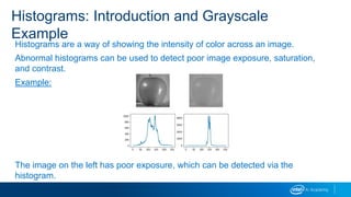


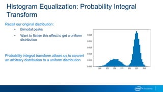
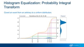
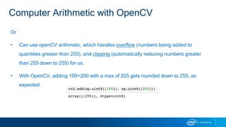
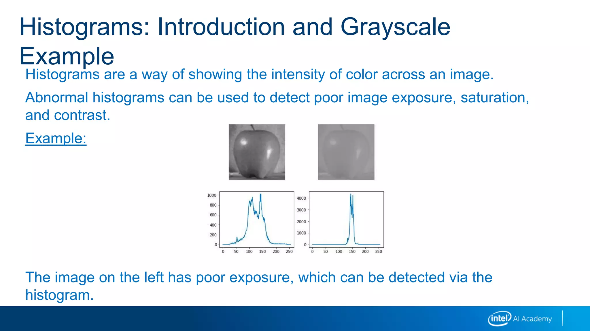
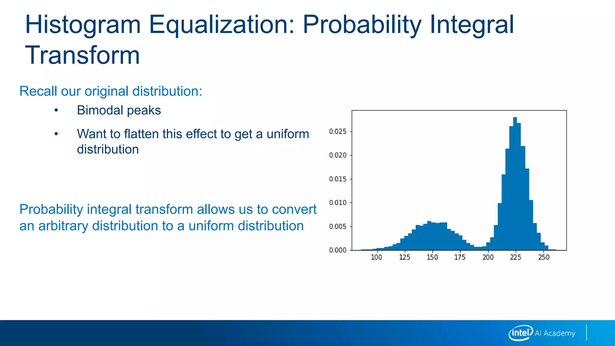
![Histogram Equalization: Probability Integral
TransformOur original is a distribution of pixel intensities.
We will use percentiles from both the arbitrary distribution and the uniform distribution
to do this conversion.
We need to know, for our input intensity x, what percentile it falls in to.
We compute the cumulative (running total) of the probabilities of the values less than x.
Once we know that, we have an output value between [0,1] or U(0,1)
We can map U(0,1) to U(0,255) to get uniformly scaled pixel intensities.
Simple linear scaling for (0,1) to (0, 255)](https://image.slidesharecdn.com/02imageprocessing-190218095646/85/02-image-processing-34-320.jpg)


![Imshow arguments
o (m,n):
Rows, columns: NOT x,y coordinates
Can (m,n,3) and (m,n,4)
Values uint8 or float in [0,1]
(m,n,3) = RGB
(m,n,4) = RGBA
A alpha
o “cmap”
Color map: can be RGB, grayscale, and so on
See upcoming slide for examples
o “vmin”, “vmax”
Used to change brightness
Display with matplotlib*: imshow](https://image.slidesharecdn.com/02imageprocessing-190218095646/75/02-image-processing-13-2048.jpg)


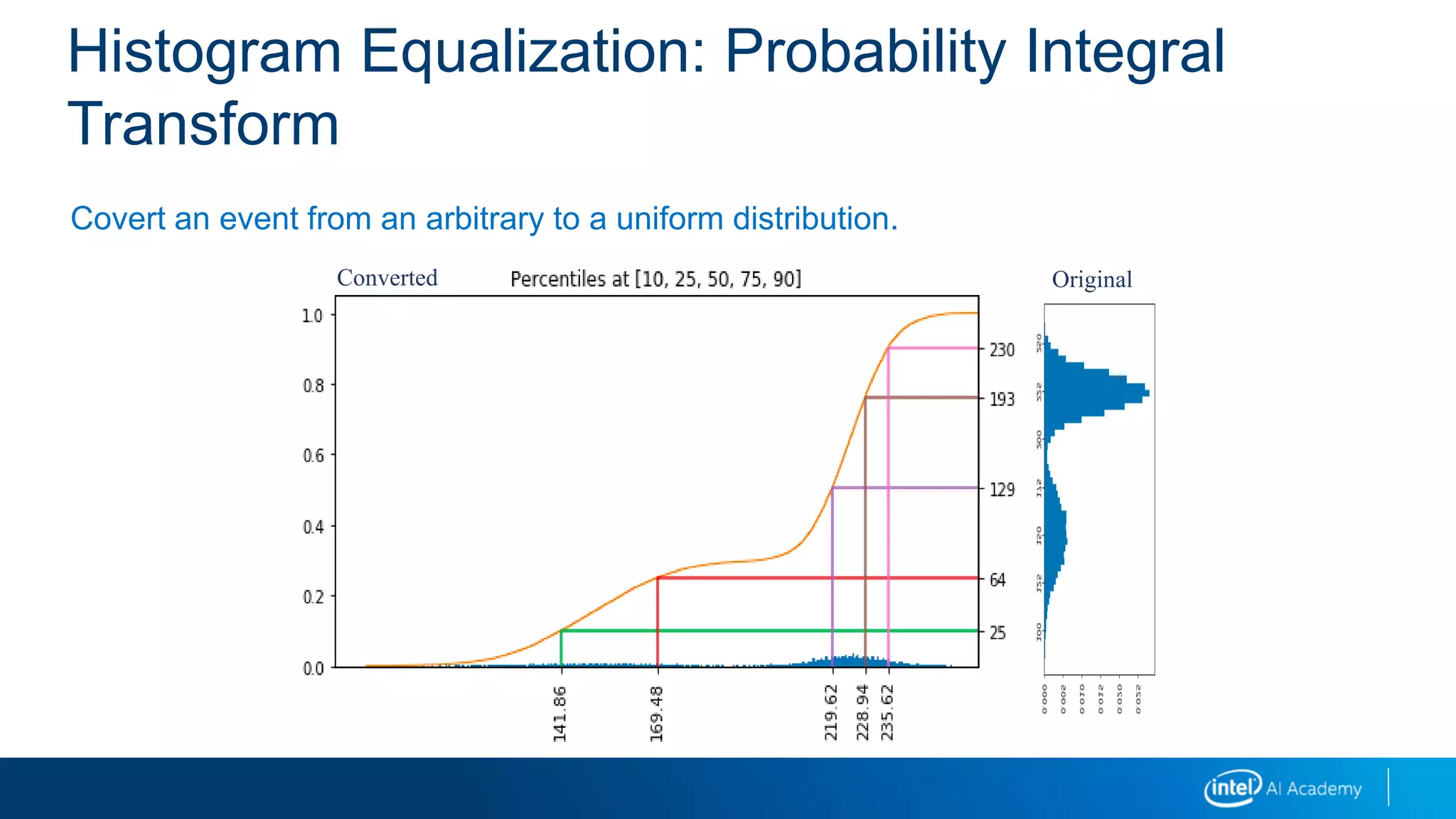
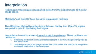
![Histogram Equalization: Probability Integral
TransformOur original is a distribution of pixel intensities.
We will use percentiles from both the arbitrary distribution and the uniform distribution
to do this conversion.
We need to know, for our input intensity x, what percentile it falls in to.
We compute the cumulative (running total) of the probabilities of the values less than x.
Once we know that, we have an output value between [0,1] or U(0,1)
We can map U(0,1) to U(0,255) to get uniformly scaled pixel intensities.
Simple linear scaling for (0,1) to (0, 255)](https://image.slidesharecdn.com/02imageprocessing-190218095646/75/02-image-processing-34-2048.jpg)