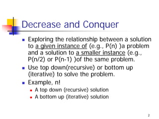
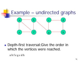
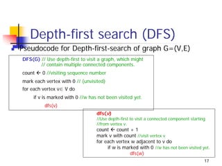
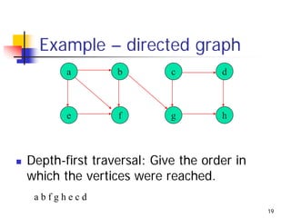
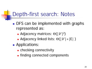
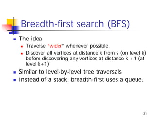
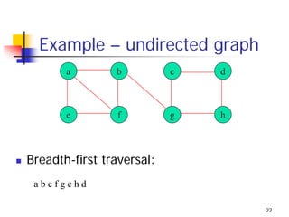
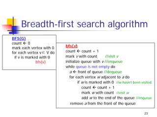
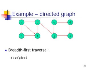
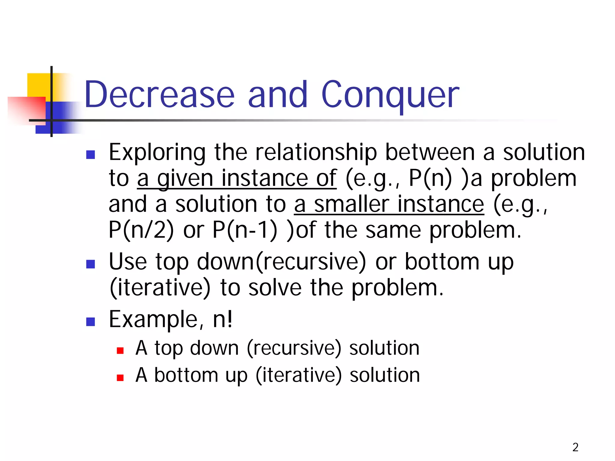
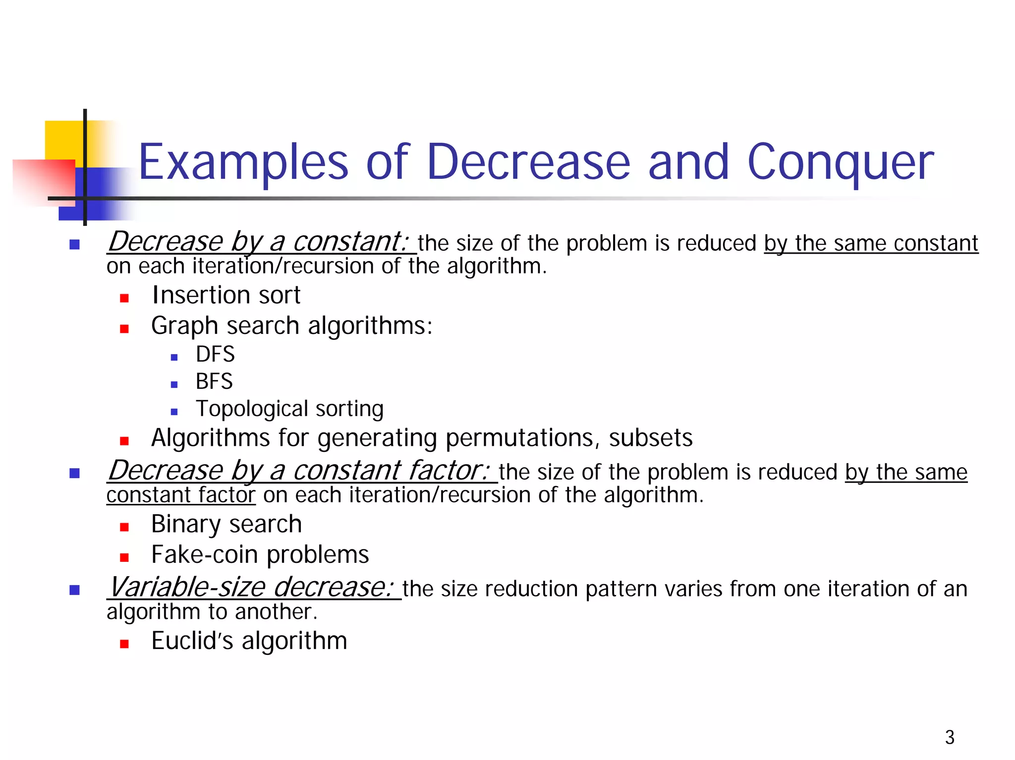
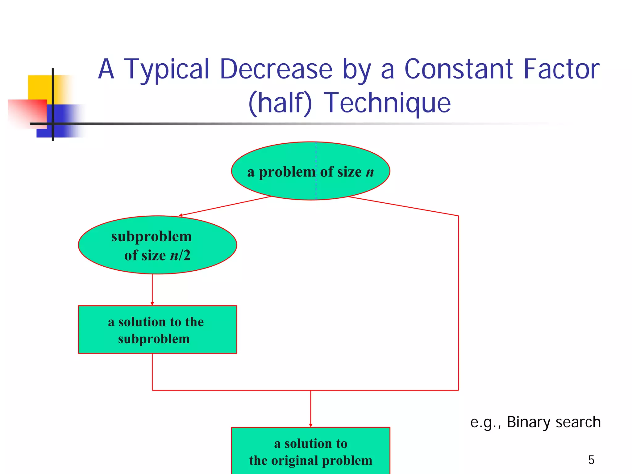
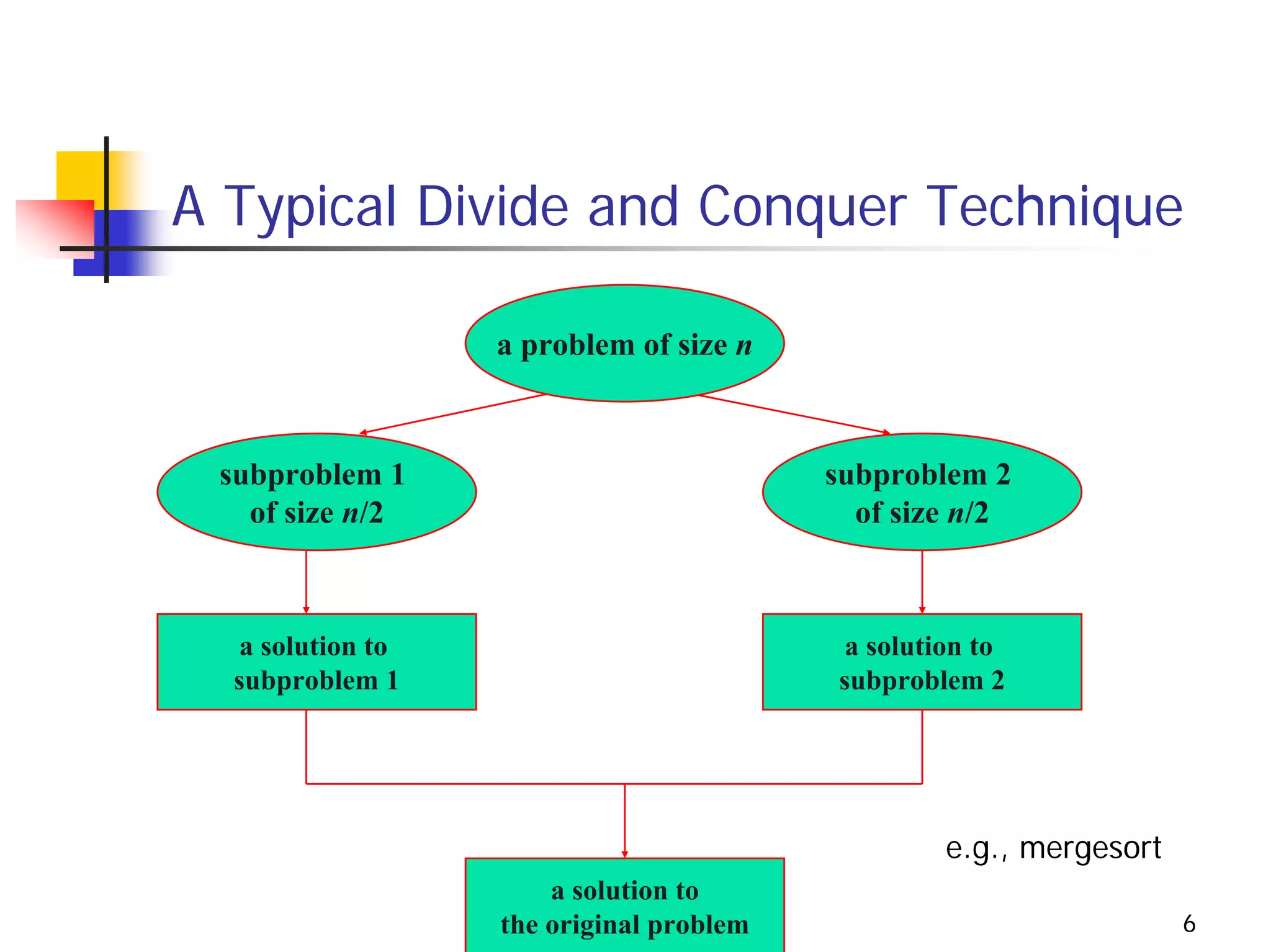
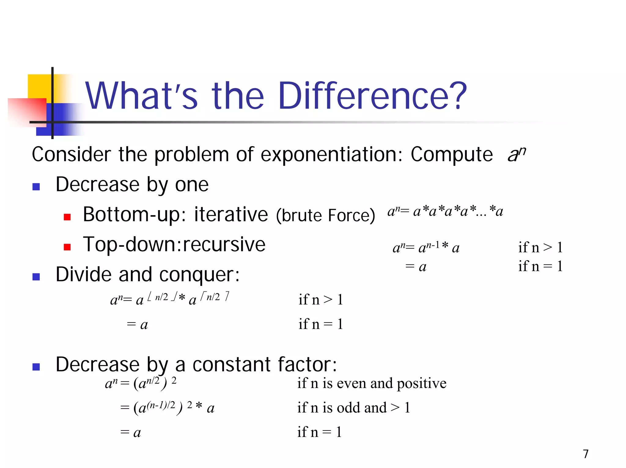
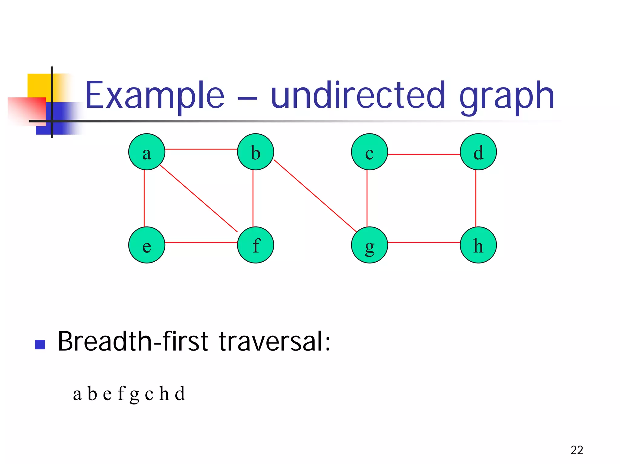
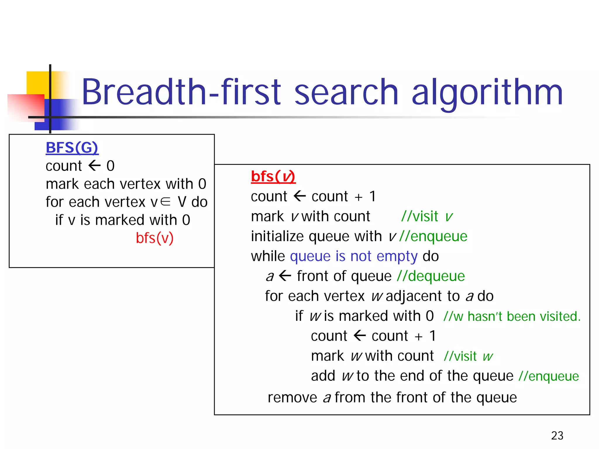
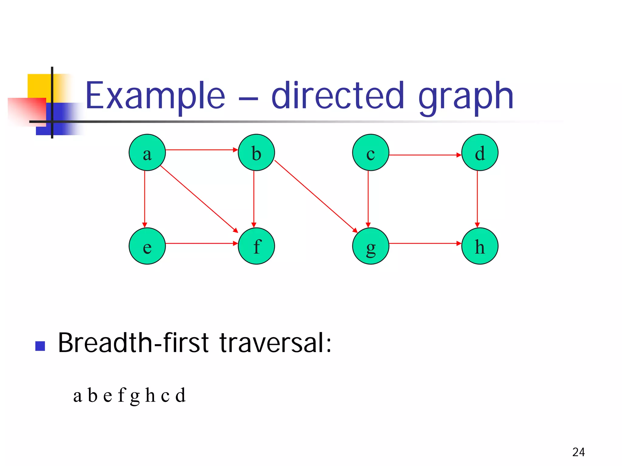
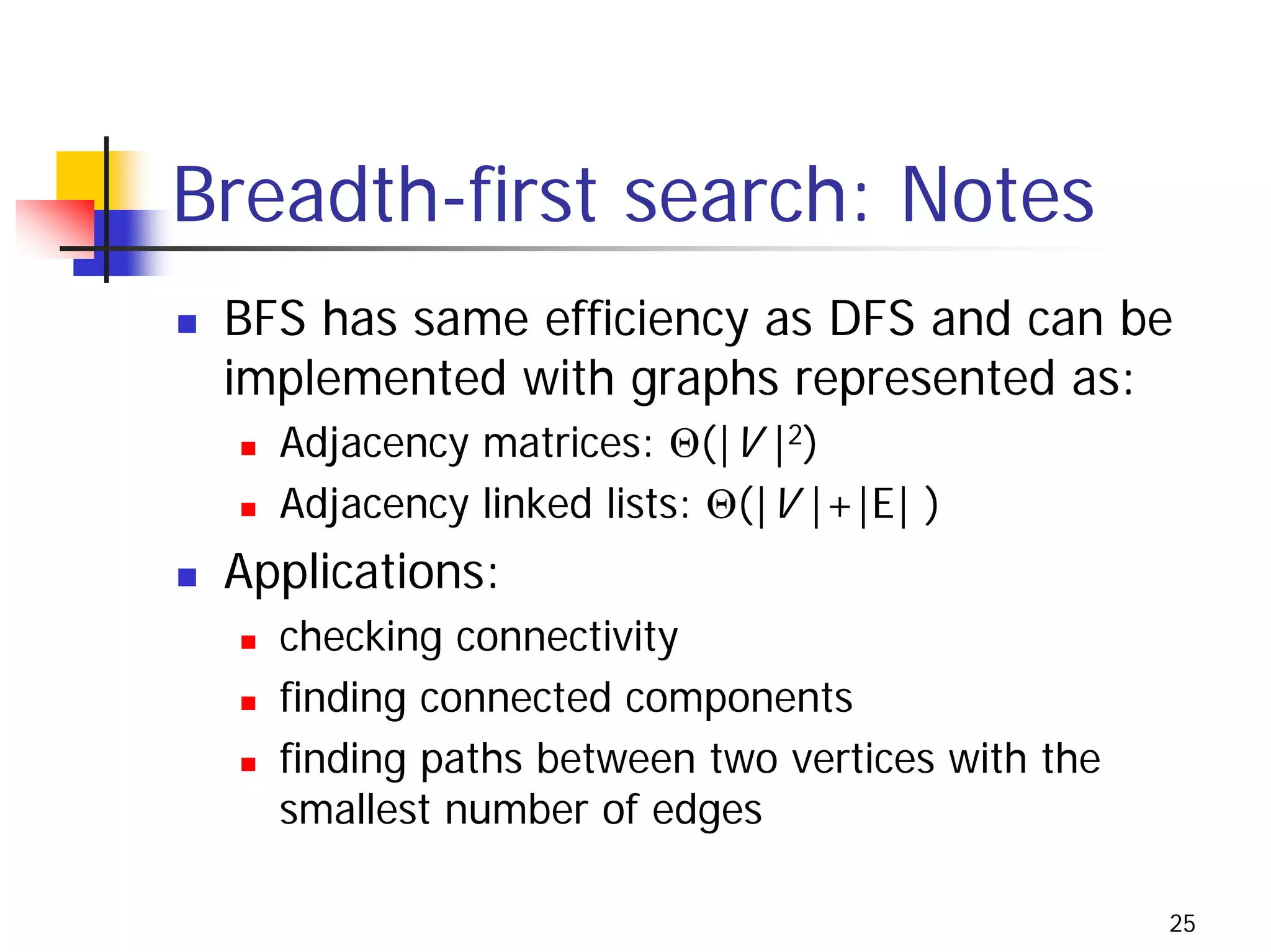
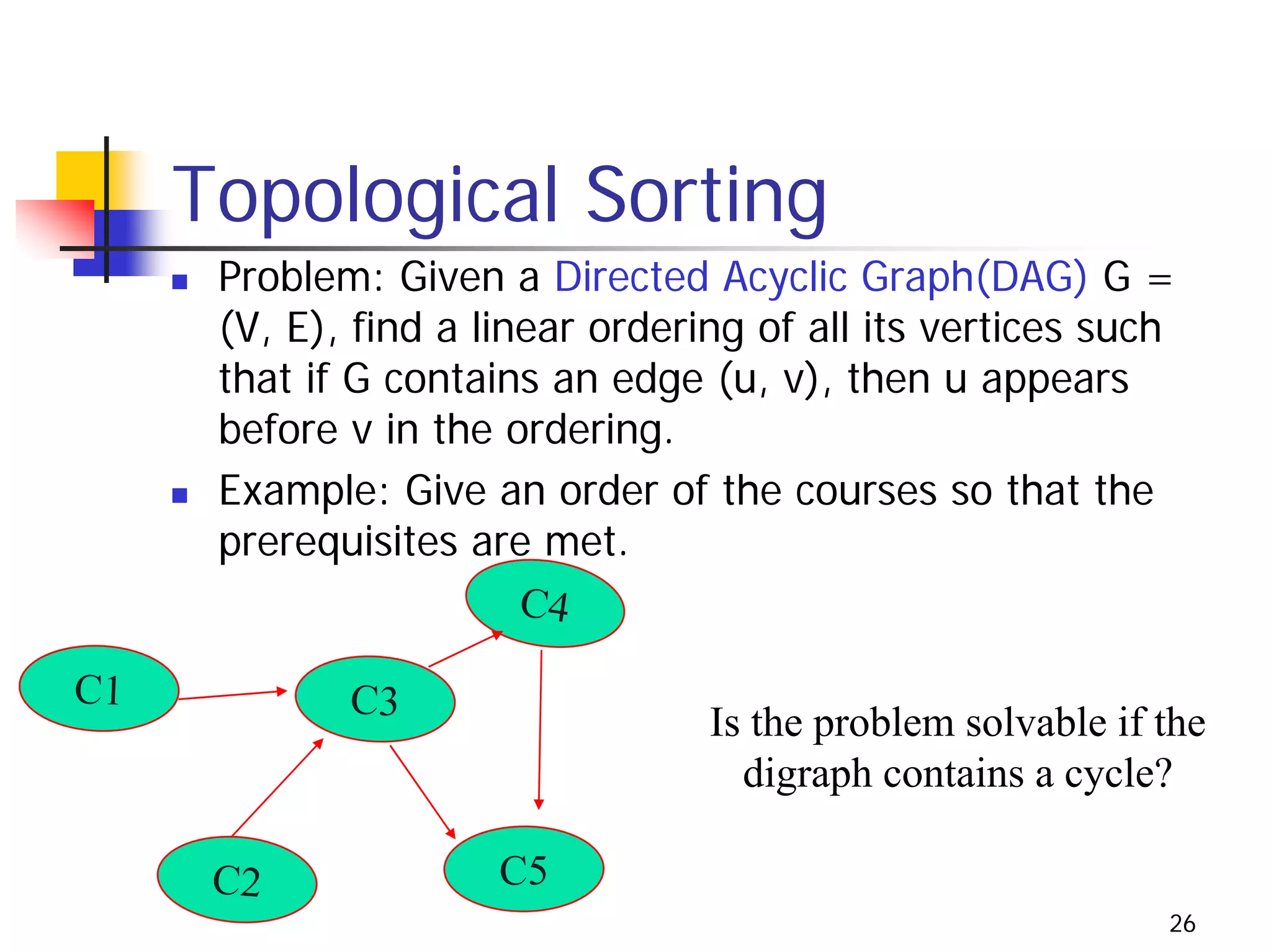
KEMBAR78
Algorithm chapter 5 | PDF
Decrease and Conquer
 Exploring the relationship between a solution
 to a given instance of (e.g., P(n) )a problem
 and a solution to a smaller instance (e.g.,
 P(n/2) or P(n-1) )of the same problem.
 Use top down(recursive) or bottom up
 (iterative) to solve the problem.
 Example, n!
   A top down (recursive) solution
   A bottom up (iterative) solution


                                            2
Examples of Decrease and Conquer
Decrease by a constant:         the size of the problem is reduced by the same constant
on each iteration/recursion of the algorithm.
    Insertion sort
    Graph search algorithms:
        DFS
        BFS
        Topological sorting
    Algorithms for generating permutations, subsets
Decrease by a constant factor:          the size of the problem is reduced by the same
constant factor on each iteration/recursion of the algorithm.
    Binary search
    Fake-coin problems
Variable-size decrease: the size reduction pattern varies from one iteration of an
algorithm to another.
    Euclid’s algorithm


                                                                                   3
A Typical Decrease by One Technique

                     a problem of size n


  subproblem
    of size n-1


 a solution to the
  subproblem


                                            e.g., n!
                         a solution to
                     the original problem              4
A Typical Decrease by a Constant Factor
            (half) Technique

                    a problem of size n


 subproblem
   of size n/2


a solution to the
  subproblem


                                           e.g., Binary search
                        a solution to
                    the original problem                    5
A Typical Divide and Conquer Technique

                   a problem of size n


 subproblem 1                             subproblem 2
   of size n/2                              of size n/2


   a solution to                           a solution to
  subproblem 1                            subproblem 2


                                                  e.g., mergesort
                       a solution to
                   the original problem                             6
What’s the Difference?
Consider the problem of exponentiation: Compute an
  Decrease by one
     Bottom-up: iterative (brute Force) an= a*a*a*a*...*a
     Top-down:recursive                  an= an-1* a      if n > 1
                                                          if n = 1
  Divide and conquer:                      =a

          an= a ⎣ n/2 ⎦ * a ⎡ n/2 ⎤   if n > 1
             =a                       if n = 1

  Decrease by a constant factor:
         an = (an/2 ) 2               if n is even and positive
            = (a(n-1)/2 ) 2 * a       if n is odd and > 1
            =a                        if n = 1
                                                                     7
Insertion Sort
 A decrease by one algorithm
   A bottom-up (iterative) solution
   A top-down (recursive) solution


                                      8
Insertion Sort: an Iterative Solution
ALGORITHM InsertionSortIter(A[0..n-1])
//An iterative implementation of insertion sort
//Input: An array A[0..n-1] of n orderable elements
//Output: Array A[0..n-1] sorted in nondecreasing order

for i    1 to n – 1 do      // i: the index of the first element of the unsorted part.
   key = A[i]
   for j    i – 1 to 0 do   // j: the index of the sorted part of the array
   if (key< A[j])           //compare the key with each element in the sorted part
         A[j+1]      A[j]
   else
         break
   A[j +1]      key         //insert the key to the sorted part of the array


                                                   Efficiency?
                                                                                     9
Insertion Sort: a Recursive Solution
ALGORITHM InsertionSortRecur(A[0..n-1], n-1)
//A recursive implementation of insertion sort
//Input: An array A[0..n-1] of n orderable elements       Index of the last element
//Output: Array A[0..n-1] sorted in nondecreasing order
if n > 1
    InsertionSortRecur(A[0..n-1], n-2)
    Insert(A[0..n-1], n-1) //insert A[n-1] to A[0..n-2]
                                              Index of the element/key to be inserted.
ALGORITHM Insert(A[0..m], m)
//Insert A[m] to the sorted subarray A[0..m-1] of A[0..n-1]
//Input: A subarray A[0..m] of A[0..n-1]
//Output: Array A[0..m] sorted in nondecreasing order
key = A[m]
for j    m – 1 to 0 do
    if (key< A[j])
          A[j+1]    A[j]                     Recurrence       relation?
    else
          break
A[j +1]     key                                                                       10
Exercises
Design a recursive decrease-by-one algorithm for
  finding the position of the largest element in an array
  of n real numbers.
Determine the time efficiency of this algorithm and
  compare it with that of the brute-force algorithm for
  the same problem.


                                                     11
Graph Traversal
 Many problems require processing all graph
 vertices in a systematic fashion

 Graph traversal algorithms:

   Depth-first search

   Breadth-first search

                                          12
Some Terminologies
Vertices and Edges
Undirected and directed graphs
Parents, children, and ancestors.
Connected graphs
  A graph is said to be connected if for every
  pair of its vertices u and v there is a path
  from u to v.


                                                 13
Graph Representation
 Adjacency matrix
    n x n boolean matrix if |V| is n.
    The element on the ith row and jth column is 1 if there’s an
    edge from ith vertex to the jth vertex; otherwise 0.
    The adjacency matrix of an undirected graph is symmetric.
    It takes |V| (comparisons) to figure out all the adjacent
    nodes of a certain node i.
 Adjacency linked lists
    A collection of linked lists, one for each vertex, that contain
    all the vertices adjacent to the list’s vertex.
 An example


                                                                14
Depth-first search
The idea
   traverse “deeper” whenever possible.
   On each iteration, the algorithm proceeds to an unvisited vertex that is
   adjacent to the one it is currently in. If there are more than more
   neighbors, break the tie by the alphabetic order of the vertices.
   When reaching a dead end ( a vertex with no adjacent unvisited vertices),
   the algorithm backs up one edge to the parent and tries to continue visiting
   unvisited vertices from there.
   The algorithm halts after backing up to the starting vertex, with the latter
   being a dead end.
Similar to preorder tree traversals
It’s convenient to use a stack to trace the operation of depth-first
search.
   Push a vertex onto the stack when the vertex is reached for the first time.
   Pop a vertex off the stack when it becomes a dead end.
An example

                                                                             15
Example – undirected graphs
       a        b         c        d


       e        f         g        h


Depth-first traversal:Give the order in
which the vertices were reached.
 abfegcdh
                                          16
Depth-first search (DFS)
Pseudocode for Depth-first-search of graph G=(V,E)
DFS(G) // Use depth-first to visit a graph, which might
       // contain multiple connected components.
count    0 //visiting sequence number
mark each vertex with 0 // (unvisited)
for each vertex v∈ V do
     if v is marked with 0 //w has not been visited yet.
          dfs(v)
                                  dfs(v)
                                  //Use depth-first to visit a connected component starting
                                  //from vertex v.
                                  count     count + 1
                                  mark v with count //visit vertex v
                                  for each vertex w adjacent to v do
                                       if w is marked with 0 //w has not been visited yet.
                                                  dfs(w)
                                                                                          17
Types of edges
 Tree edges: edges comprising forest

 Back edges: edges to ancestor nodes

 Forward edges: edges to descendants
 (digraphs only)

 Cross edges: none of the above

                                       18
Example – directed graph
       a        b         c        d


       e        f         g        h


Depth-first traversal: Give the order in
which the vertices were reached.
 abfghecd
                                           19
Depth-first search: Notes
 DFS can be implemented with graphs
 represented as:
   Adjacency matrices: Θ(|V |2)
   Adjacency linked lists: Θ(|V |+|E| )
 Applications:
   checking connectivity
   finding connected components


                                          20
Breadth-first search (BFS)
The idea
  Traverse “wider” whenever possible.
  Discover all vertices at distance k from s (on level k)
  before discovering any vertices at distance k +1 (at
  level k+1)
Similar to level-by-level tree traversals
Instead of a stack, breadth-first uses a queue.


                                                       21
Example – undirected graph
       a        b          c   d


       e        f          g   h


Breadth-first traversal:
 abefgchd

                                   22
Breadth-first search algorithm
BFS(G)
count      0
mark each vertex with 0   bfs(v)
for each vertex v∈ V do   count        count + 1
  if v is marked with 0   mark v with count         //visit v
               bfs(v)     initialize queue with v //enqueue
                          while queue is not empty do
                             a      front of queue //dequeue
                             for each vertex w adjacent to a do
                                   if w is marked with 0 //w hasn’t been visited.
                                      count     count + 1
                                      mark w with count //visit w
                                      add w to the end of the queue //enqueue
                              remove a from the front of the queue

                                                                           23
Example – directed graph
       a        b          c   d


       e        f          g   h


Breadth-first traversal:
 abefghcd

                                   24
Breadth-first search: Notes
 BFS has same efficiency as DFS and can be
 implemented with graphs represented as:
   Adjacency matrices: Θ(|V |2)
   Adjacency linked lists: Θ(|V |+|E| )
 Applications:
   checking connectivity
   finding connected components
   finding paths between two vertices with the
   smallest number of edges

                                                 25
Topological Sorting
      Problem: Given a Directed Acyclic Graph(DAG) G =
      (V, E), find a linear ordering of all its vertices such
      that if G contains an edge (u, v), then u appears
      before v in the ordering.
      Example: Give an order of the courses so that the
      prerequisites are met.
                        C4

C1           C3
                                  Is the problem solvable if the
                                    digraph contains a cycle?

      C2              C5
                                                             26
The DFS-Based Algorithm
DFS-based algorithm: (2 orderings exist in the DFS)
  DFS traversal noting the order in which vertices are
  popped off stack (the order in which the dead end
  vertices appear)
  Reverse the above order.
Questions
  Can we use the order in which vertices are pushed onto
  the DFS stack (instead of the order they are popped off it)
  to solve the topological sorting problem?
  Does it matter from which node we start?
  Θ(|V |+|E| ) using adjacency linked lists

                                                         27
Example: Scheduling with Task Dependencies

Task        Number   Depends                            Wake up 1
                     on
Wake up     1        --
Dress       2        7,8                                               Make      Make
                                                                      coffee 5   toast 6
Eat         3        5, 6                        Shower 7
                               Choose
breakfast                      clothes 8
Leave       4        2, 3
                                                                  Eat
Make        5        1
                                                               breakfast 3
coffee                                     Dress 2
Make        6        1
toast
Shower      7        1                               Leave 4
Choose      8        1
clothes
                                                                                 28
The Source Removal Algorithms
Source removal algorithm
    Based on a direct implementation of the
    decrease-by-one techniques.
    Repeatedly identify and remove a source
    vertex, ie, a vertex that has no incoming edges,
    and delete it along with all the edges outgoing
    from it.


                                                  29
Exercises
 Problem 1, Exercise 5.2
 Problem 1, Exercise 5.3
 Problem 5, Exercise 5.3


                           30

Algorithm chapter 5

  • 1.
  • 2.
    Decrease and Conquer Exploring the relationship between a solution to a given instance of (e.g., P(n) )a problem and a solution to a smaller instance (e.g., P(n/2) or P(n-1) )of the same problem. Use top down(recursive) or bottom up (iterative) to solve the problem. Example, n! A top down (recursive) solution A bottom up (iterative) solution 2
  • 3.
    Examples of Decreaseand Conquer Decrease by a constant: the size of the problem is reduced by the same constant on each iteration/recursion of the algorithm. Insertion sort Graph search algorithms: DFS BFS Topological sorting Algorithms for generating permutations, subsets Decrease by a constant factor: the size of the problem is reduced by the same constant factor on each iteration/recursion of the algorithm. Binary search Fake-coin problems Variable-size decrease: the size reduction pattern varies from one iteration of an algorithm to another. Euclid’s algorithm 3
  • 4.
    A Typical Decreaseby One Technique a problem of size n subproblem of size n-1 a solution to the subproblem e.g., n! a solution to the original problem 4
  • 5.
    A Typical Decreaseby a Constant Factor (half) Technique a problem of size n subproblem of size n/2 a solution to the subproblem e.g., Binary search a solution to the original problem 5
  • 6.
    A Typical Divideand Conquer Technique a problem of size n subproblem 1 subproblem 2 of size n/2 of size n/2 a solution to a solution to subproblem 1 subproblem 2 e.g., mergesort a solution to the original problem 6
  • 7.
    What’s the Difference? Considerthe problem of exponentiation: Compute an Decrease by one Bottom-up: iterative (brute Force) an= a*a*a*a*...*a Top-down:recursive an= an-1* a if n > 1 if n = 1 Divide and conquer: =a an= a ⎣ n/2 ⎦ * a ⎡ n/2 ⎤ if n > 1 =a if n = 1 Decrease by a constant factor: an = (an/2 ) 2 if n is even and positive = (a(n-1)/2 ) 2 * a if n is odd and > 1 =a if n = 1 7
  • 8.
    Insertion Sort Adecrease by one algorithm A bottom-up (iterative) solution A top-down (recursive) solution 8
  • 9.
    Insertion Sort: anIterative Solution ALGORITHM InsertionSortIter(A[0..n-1]) //An iterative implementation of insertion sort //Input: An array A[0..n-1] of n orderable elements //Output: Array A[0..n-1] sorted in nondecreasing order for i 1 to n – 1 do // i: the index of the first element of the unsorted part. key = A[i] for j i – 1 to 0 do // j: the index of the sorted part of the array if (key< A[j]) //compare the key with each element in the sorted part A[j+1] A[j] else break A[j +1] key //insert the key to the sorted part of the array Efficiency? 9
  • 10.
    Insertion Sort: aRecursive Solution ALGORITHM InsertionSortRecur(A[0..n-1], n-1) //A recursive implementation of insertion sort //Input: An array A[0..n-1] of n orderable elements Index of the last element //Output: Array A[0..n-1] sorted in nondecreasing order if n > 1 InsertionSortRecur(A[0..n-1], n-2) Insert(A[0..n-1], n-1) //insert A[n-1] to A[0..n-2] Index of the element/key to be inserted. ALGORITHM Insert(A[0..m], m) //Insert A[m] to the sorted subarray A[0..m-1] of A[0..n-1] //Input: A subarray A[0..m] of A[0..n-1] //Output: Array A[0..m] sorted in nondecreasing order key = A[m] for j m – 1 to 0 do if (key< A[j]) A[j+1] A[j] Recurrence relation? else break A[j +1] key 10
  • 11.
    Exercises Design a recursivedecrease-by-one algorithm for finding the position of the largest element in an array of n real numbers. Determine the time efficiency of this algorithm and compare it with that of the brute-force algorithm for the same problem. 11
  • 12.
    Graph Traversal Manyproblems require processing all graph vertices in a systematic fashion Graph traversal algorithms: Depth-first search Breadth-first search 12
  • 13.
    Some Terminologies Vertices andEdges Undirected and directed graphs Parents, children, and ancestors. Connected graphs A graph is said to be connected if for every pair of its vertices u and v there is a path from u to v. 13
  • 14.
    Graph Representation Adjacencymatrix n x n boolean matrix if |V| is n. The element on the ith row and jth column is 1 if there’s an edge from ith vertex to the jth vertex; otherwise 0. The adjacency matrix of an undirected graph is symmetric. It takes |V| (comparisons) to figure out all the adjacent nodes of a certain node i. Adjacency linked lists A collection of linked lists, one for each vertex, that contain all the vertices adjacent to the list’s vertex. An example 14
  • 15.
    Depth-first search The idea traverse “deeper” whenever possible. On each iteration, the algorithm proceeds to an unvisited vertex that is adjacent to the one it is currently in. If there are more than more neighbors, break the tie by the alphabetic order of the vertices. When reaching a dead end ( a vertex with no adjacent unvisited vertices), the algorithm backs up one edge to the parent and tries to continue visiting unvisited vertices from there. The algorithm halts after backing up to the starting vertex, with the latter being a dead end. Similar to preorder tree traversals It’s convenient to use a stack to trace the operation of depth-first search. Push a vertex onto the stack when the vertex is reached for the first time. Pop a vertex off the stack when it becomes a dead end. An example 15
  • 16.
    Example – undirectedgraphs a b c d e f g h Depth-first traversal:Give the order in which the vertices were reached. abfegcdh 16
  • 17.
    Depth-first search (DFS) Pseudocodefor Depth-first-search of graph G=(V,E) DFS(G) // Use depth-first to visit a graph, which might // contain multiple connected components. count 0 //visiting sequence number mark each vertex with 0 // (unvisited) for each vertex v∈ V do if v is marked with 0 //w has not been visited yet. dfs(v) dfs(v) //Use depth-first to visit a connected component starting //from vertex v. count count + 1 mark v with count //visit vertex v for each vertex w adjacent to v do if w is marked with 0 //w has not been visited yet. dfs(w) 17
  • 18.
    Types of edges Tree edges: edges comprising forest Back edges: edges to ancestor nodes Forward edges: edges to descendants (digraphs only) Cross edges: none of the above 18
  • 19.
    Example – directedgraph a b c d e f g h Depth-first traversal: Give the order in which the vertices were reached. abfghecd 19
  • 20.
    Depth-first search: Notes DFS can be implemented with graphs represented as: Adjacency matrices: Θ(|V |2) Adjacency linked lists: Θ(|V |+|E| ) Applications: checking connectivity finding connected components 20
  • 21.
    Breadth-first search (BFS) Theidea Traverse “wider” whenever possible. Discover all vertices at distance k from s (on level k) before discovering any vertices at distance k +1 (at level k+1) Similar to level-by-level tree traversals Instead of a stack, breadth-first uses a queue. 21
  • 22.
    Example – undirectedgraph a b c d e f g h Breadth-first traversal: abefgchd 22
  • 23.
    Breadth-first search algorithm BFS(G) count 0 mark each vertex with 0 bfs(v) for each vertex v∈ V do count count + 1 if v is marked with 0 mark v with count //visit v bfs(v) initialize queue with v //enqueue while queue is not empty do a front of queue //dequeue for each vertex w adjacent to a do if w is marked with 0 //w hasn’t been visited. count count + 1 mark w with count //visit w add w to the end of the queue //enqueue remove a from the front of the queue 23
  • 24.
    Example – directedgraph a b c d e f g h Breadth-first traversal: abefghcd 24
  • 25.
    Breadth-first search: Notes BFS has same efficiency as DFS and can be implemented with graphs represented as: Adjacency matrices: Θ(|V |2) Adjacency linked lists: Θ(|V |+|E| ) Applications: checking connectivity finding connected components finding paths between two vertices with the smallest number of edges 25
  • 26.
    Topological Sorting Problem: Given a Directed Acyclic Graph(DAG) G = (V, E), find a linear ordering of all its vertices such that if G contains an edge (u, v), then u appears before v in the ordering. Example: Give an order of the courses so that the prerequisites are met. C4 C1 C3 Is the problem solvable if the digraph contains a cycle? C2 C5 26
  • 27.
    The DFS-Based Algorithm DFS-basedalgorithm: (2 orderings exist in the DFS) DFS traversal noting the order in which vertices are popped off stack (the order in which the dead end vertices appear) Reverse the above order. Questions Can we use the order in which vertices are pushed onto the DFS stack (instead of the order they are popped off it) to solve the topological sorting problem? Does it matter from which node we start? Θ(|V |+|E| ) using adjacency linked lists 27
  • 28.
    Example: Scheduling withTask Dependencies Task Number Depends Wake up 1 on Wake up 1 -- Dress 2 7,8 Make Make coffee 5 toast 6 Eat 3 5, 6 Shower 7 Choose breakfast clothes 8 Leave 4 2, 3 Eat Make 5 1 breakfast 3 coffee Dress 2 Make 6 1 toast Shower 7 1 Leave 4 Choose 8 1 clothes 28
  • 29.
    The Source RemovalAlgorithms Source removal algorithm Based on a direct implementation of the decrease-by-one techniques. Repeatedly identify and remove a source vertex, ie, a vertex that has no incoming edges, and delete it along with all the edges outgoing from it. 29
  • 30.
    Exercises Problem 1,Exercise 5.2 Problem 1, Exercise 5.3 Problem 5, Exercise 5.3 30