This document provides an overview of key algorithm analysis concepts including:
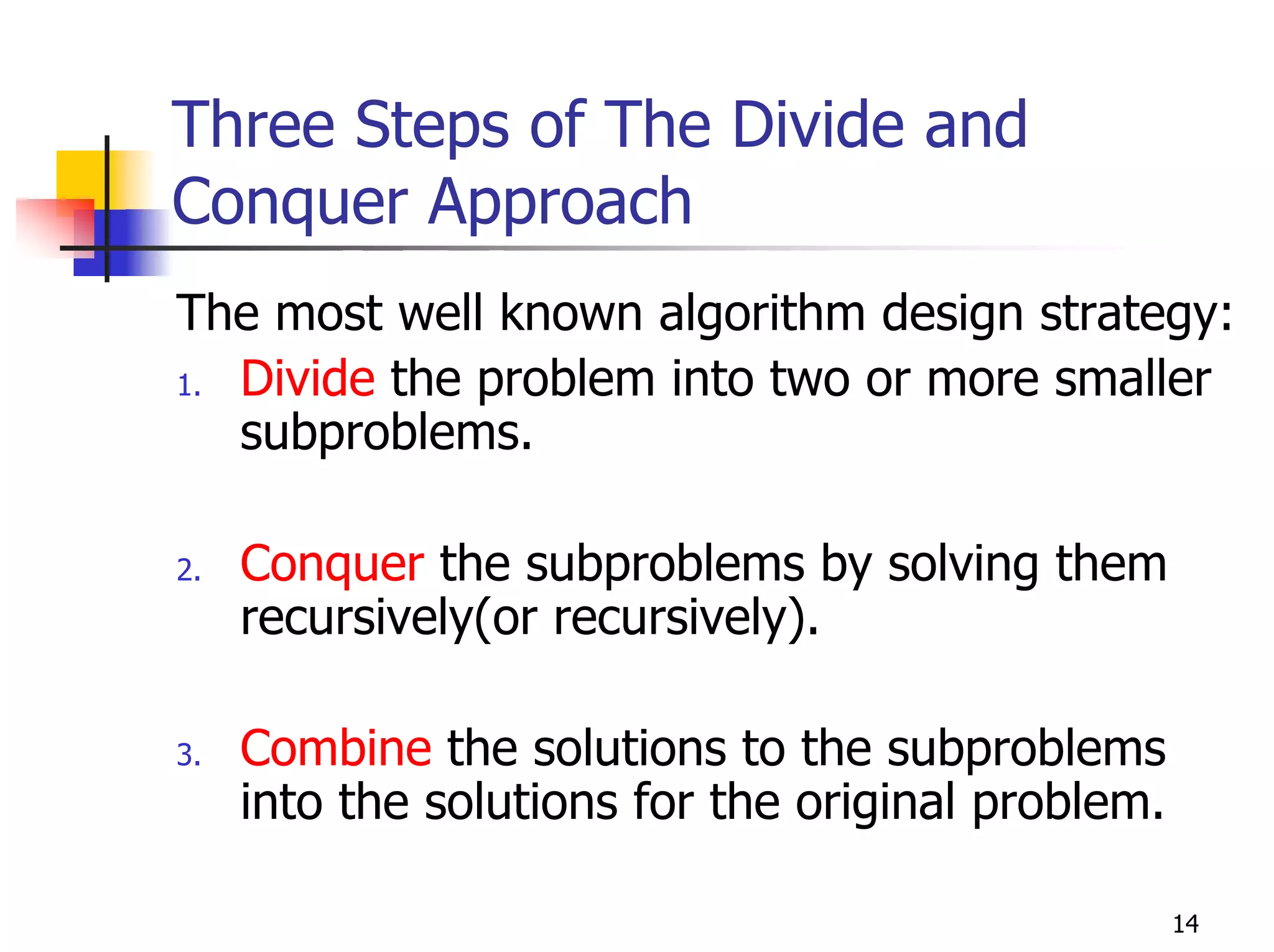
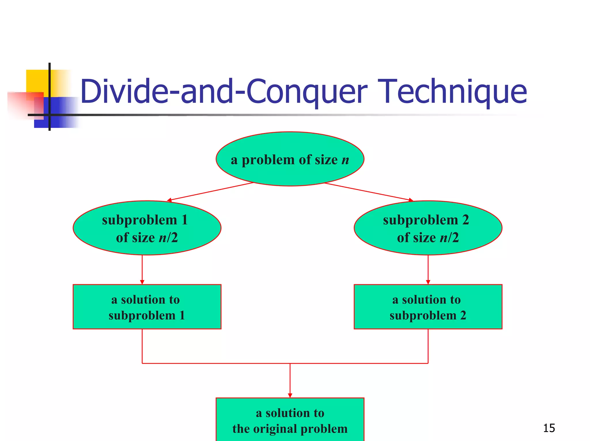
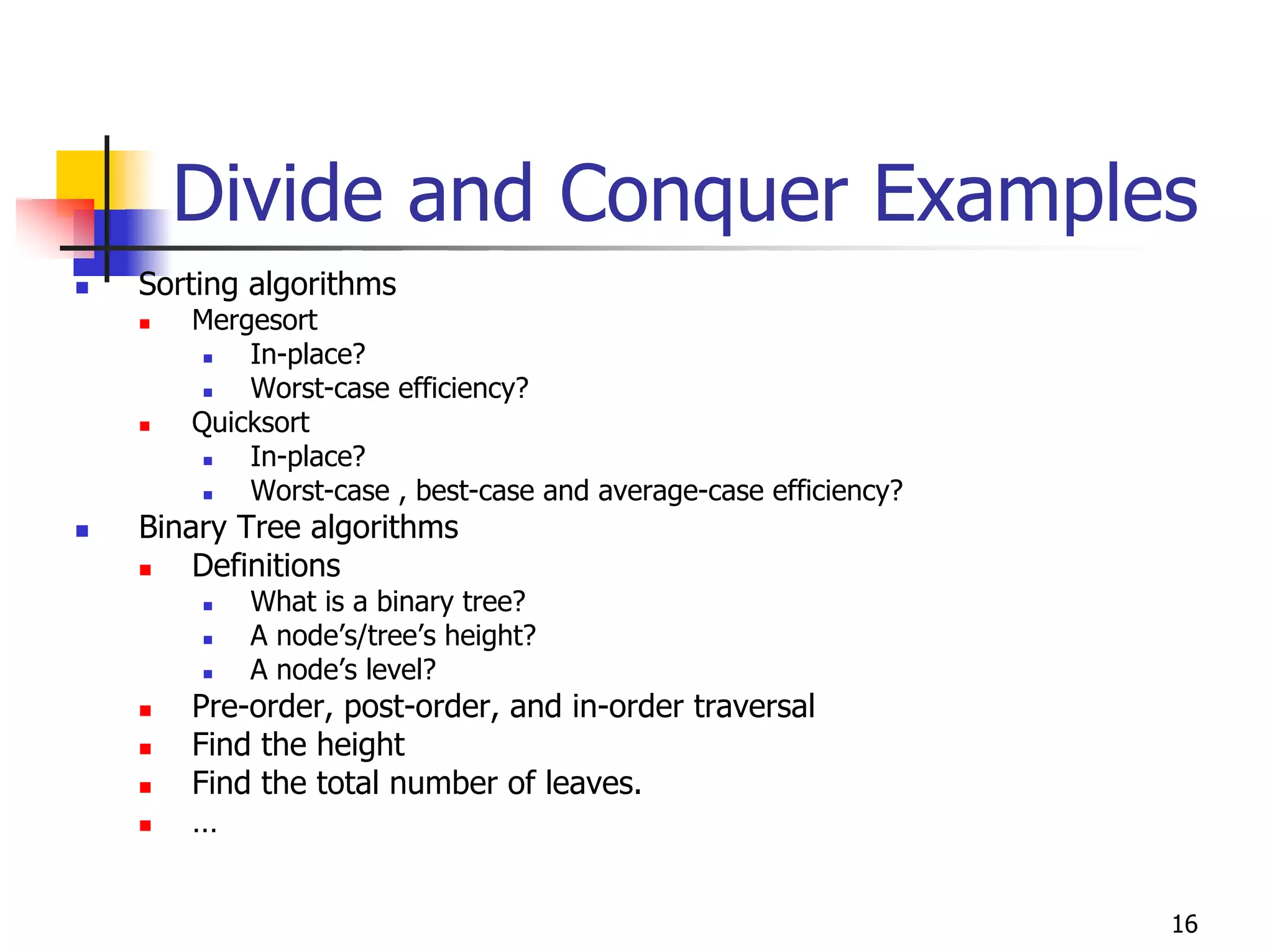
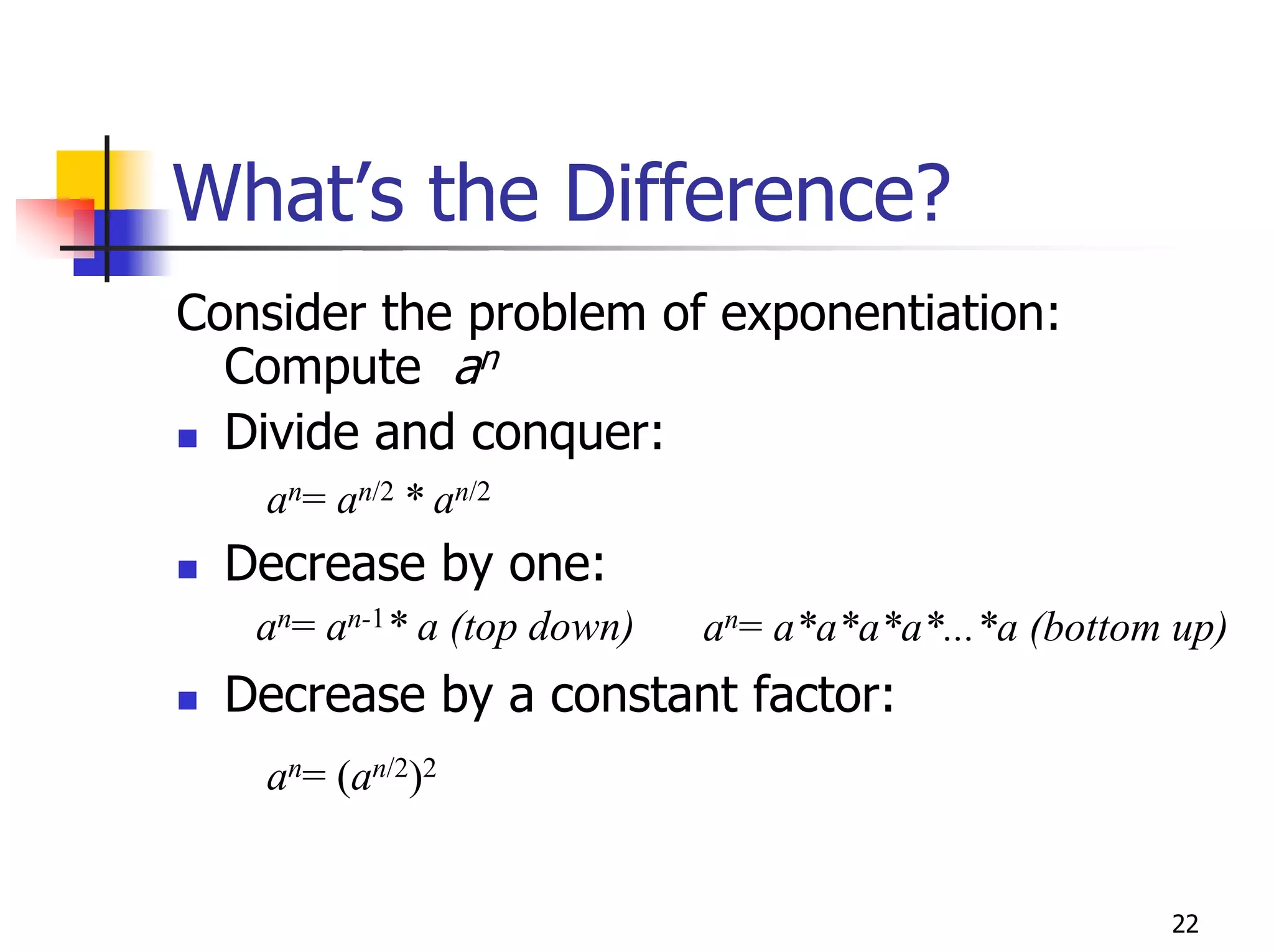
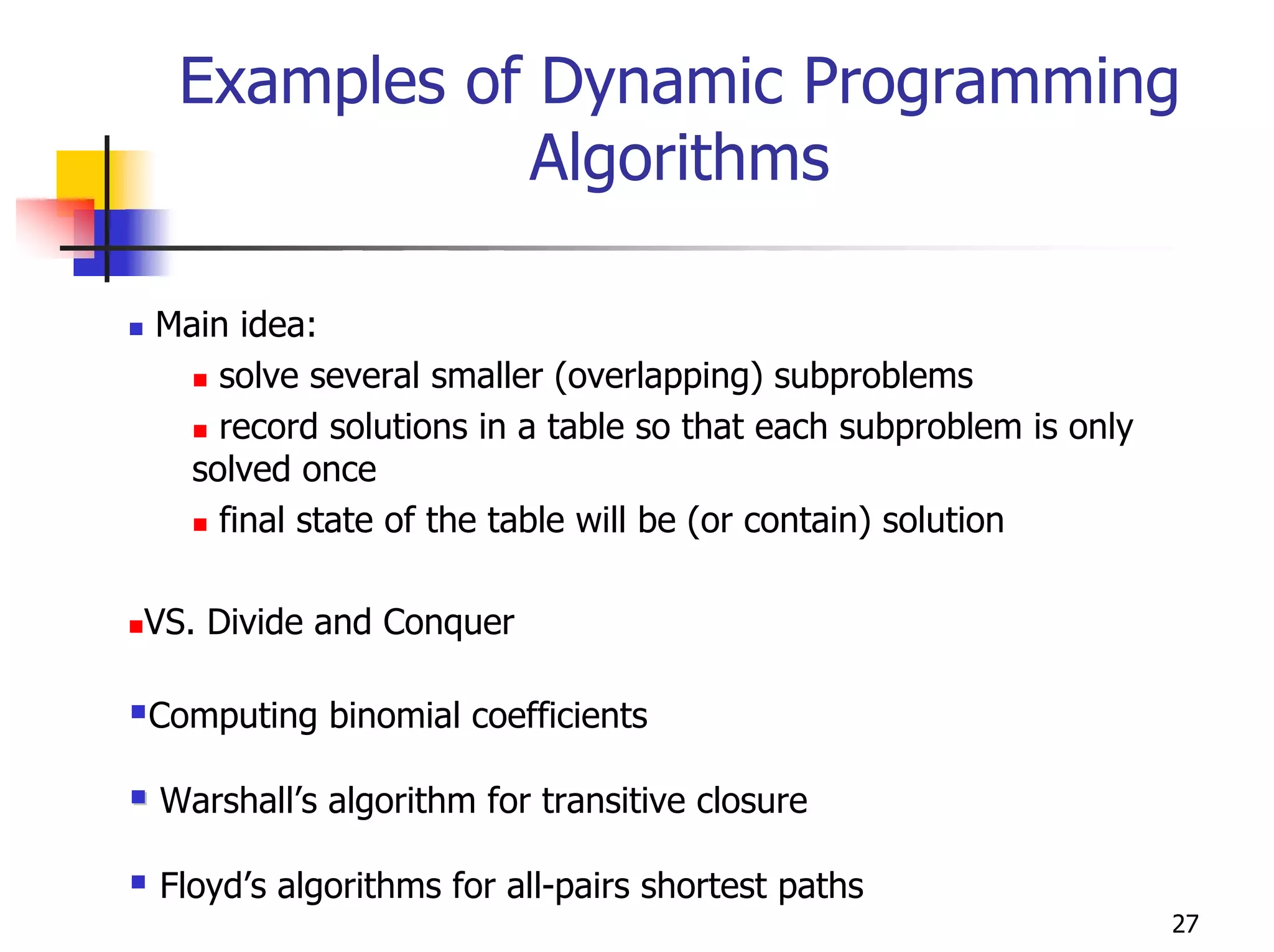
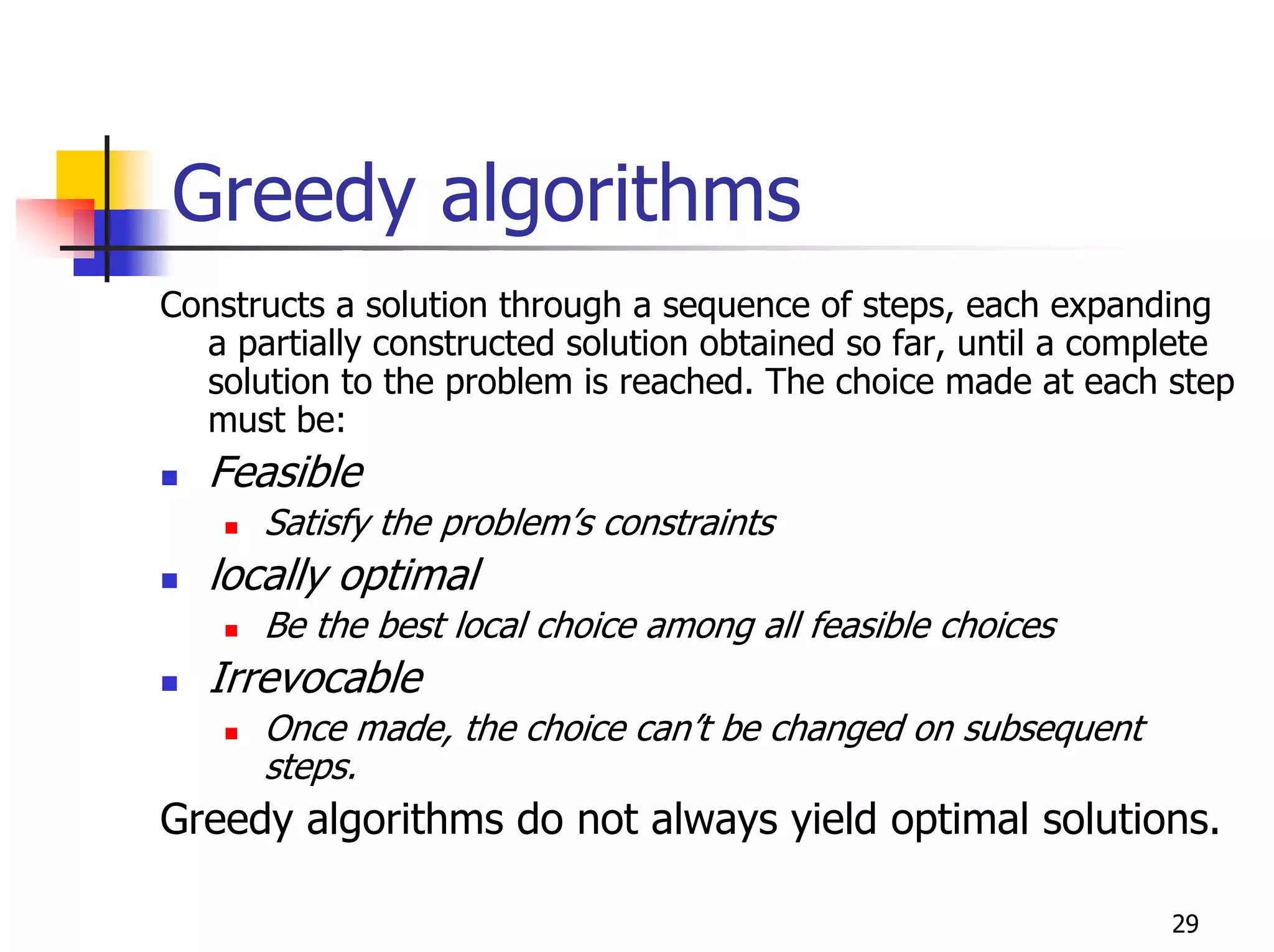
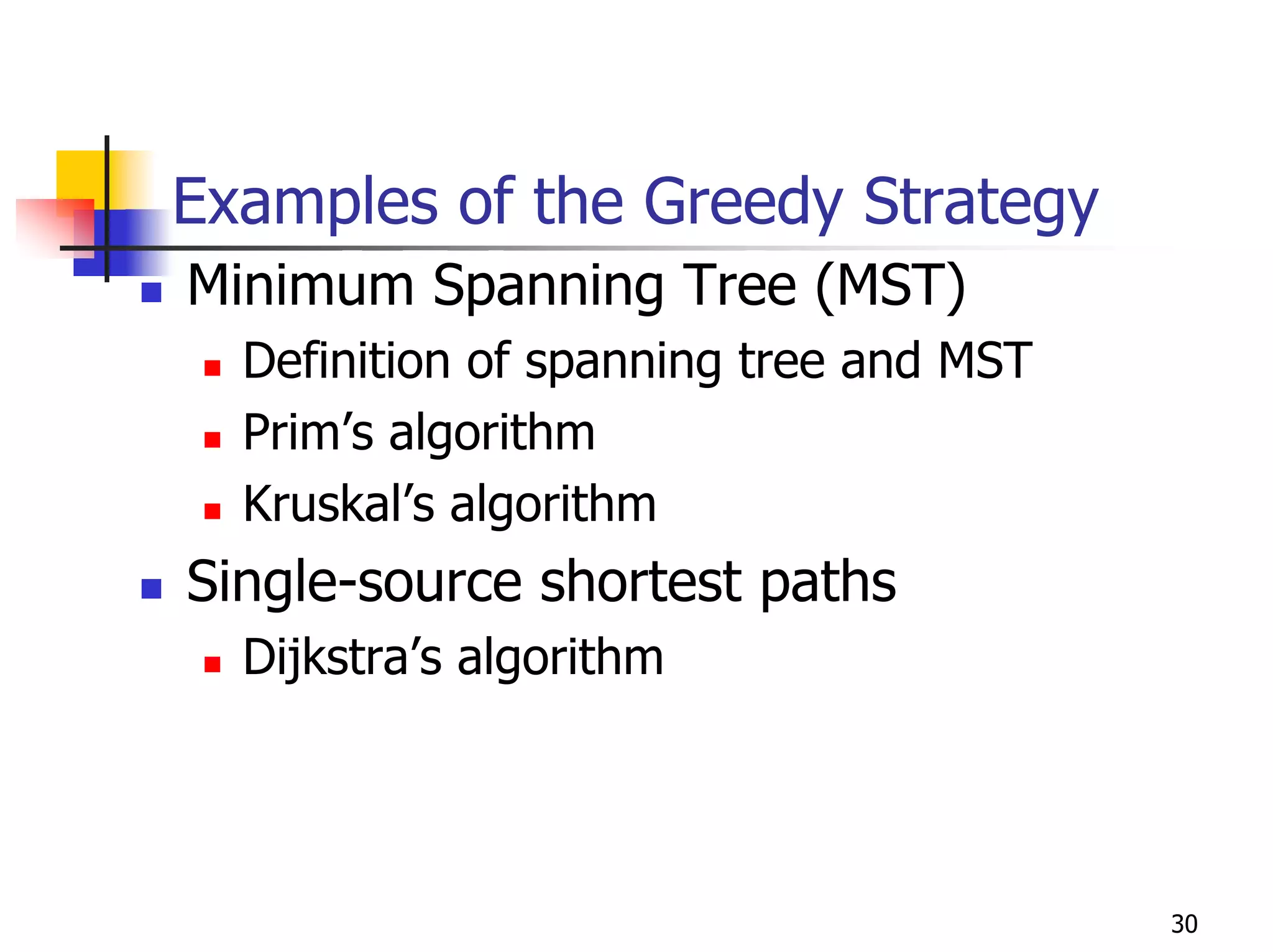
- Common algorithmic techniques like divide-and-conquer, dynamic programming, and greedy algorithms.
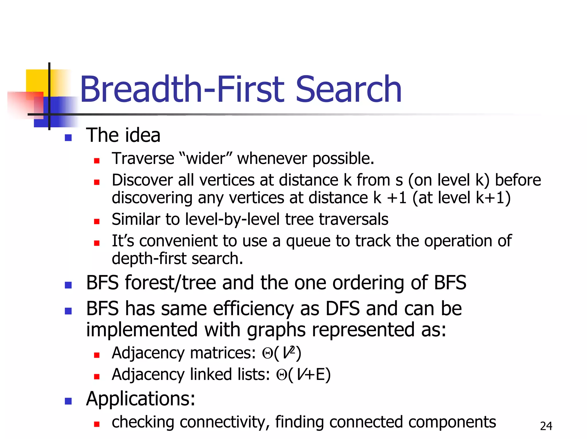
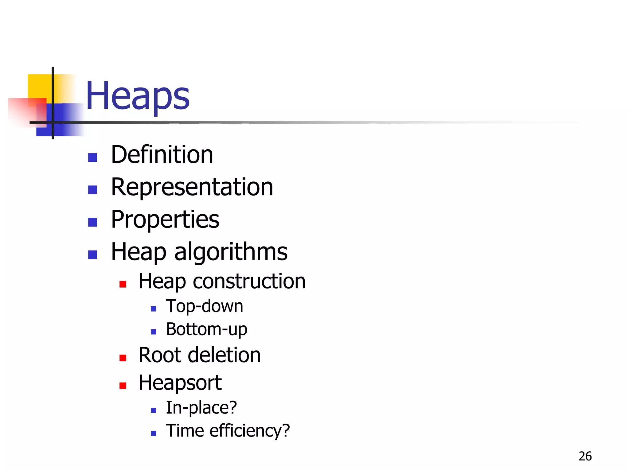
- Data structures like heaps, graphs, and trees.
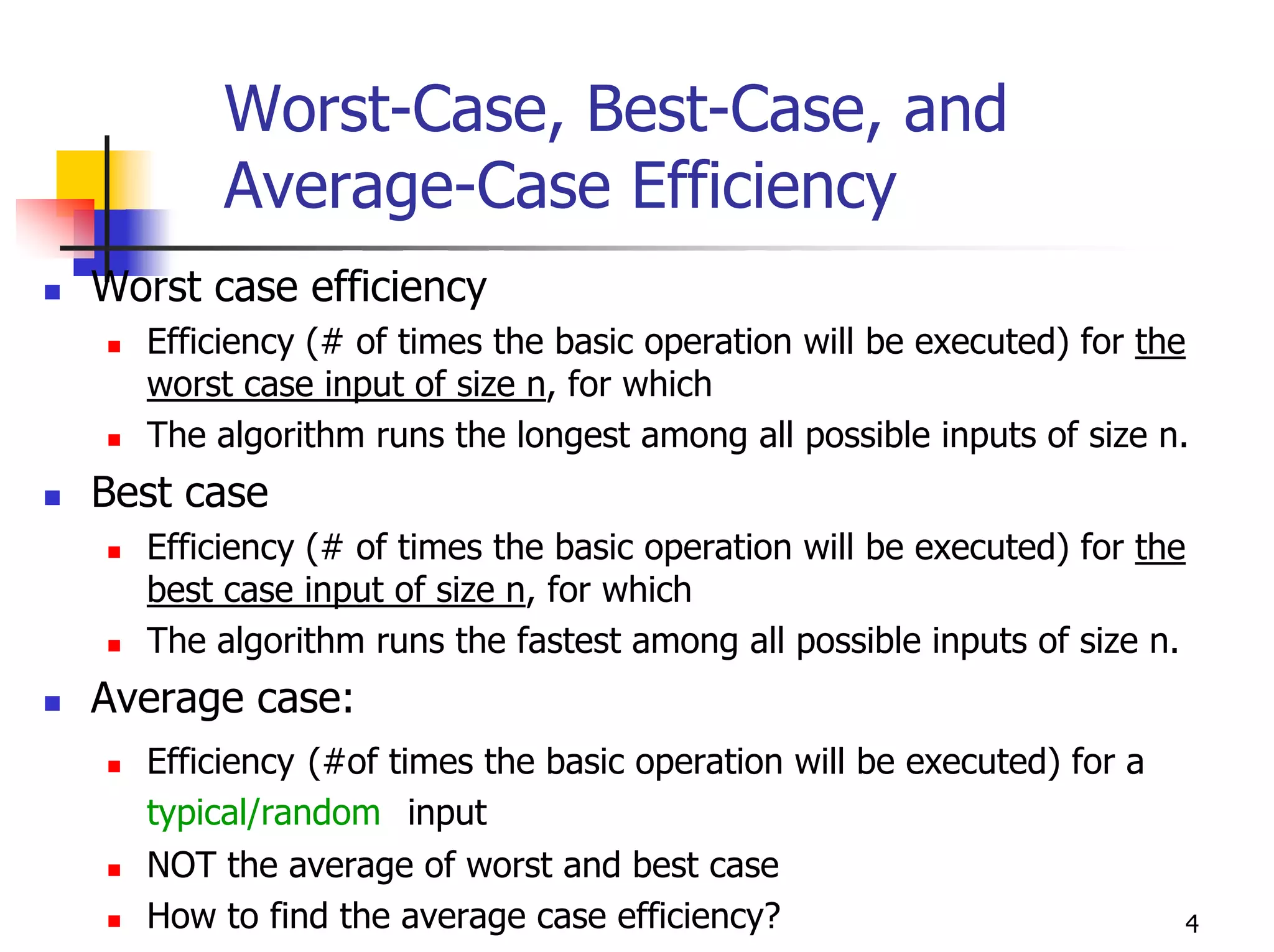
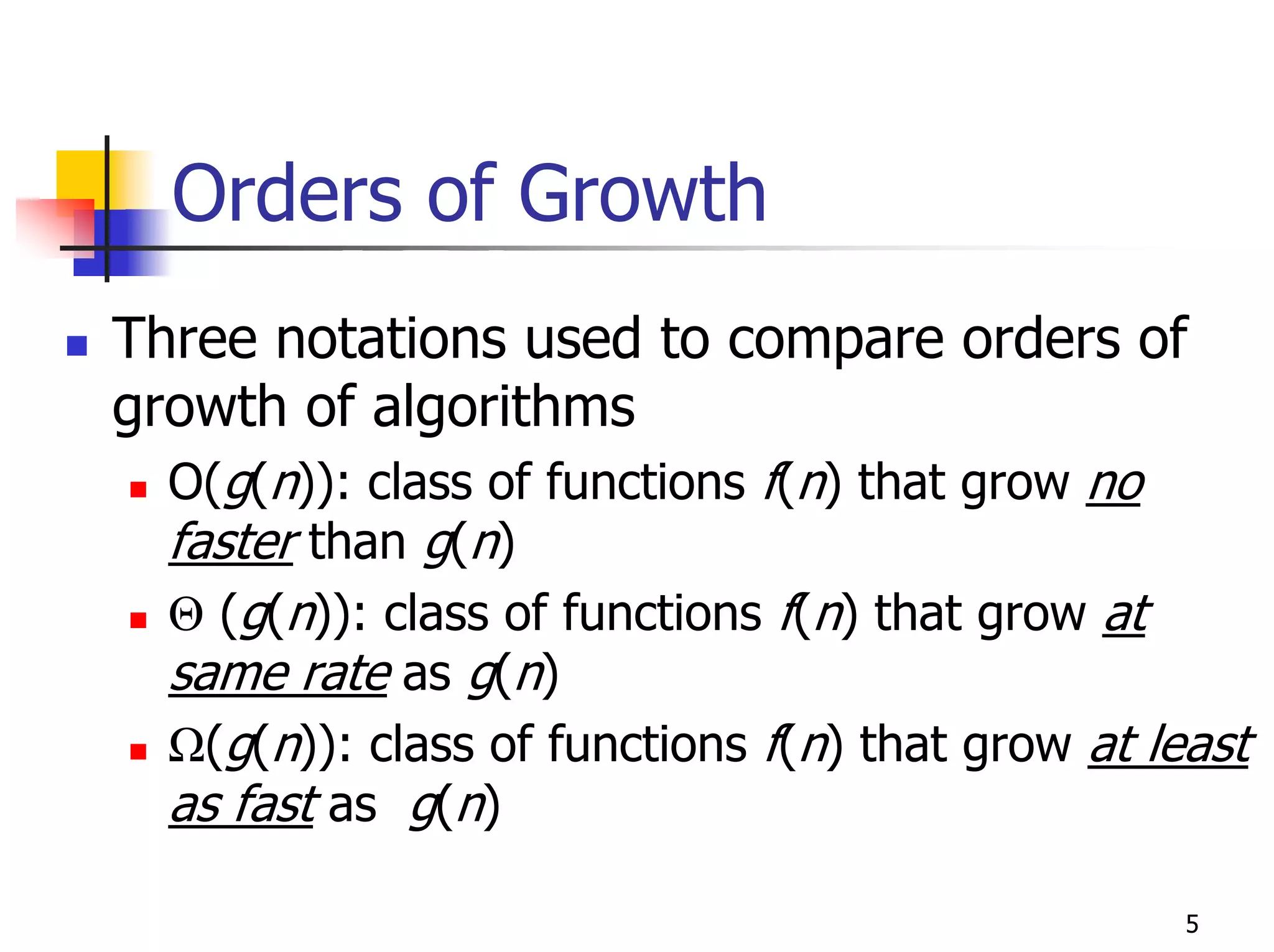
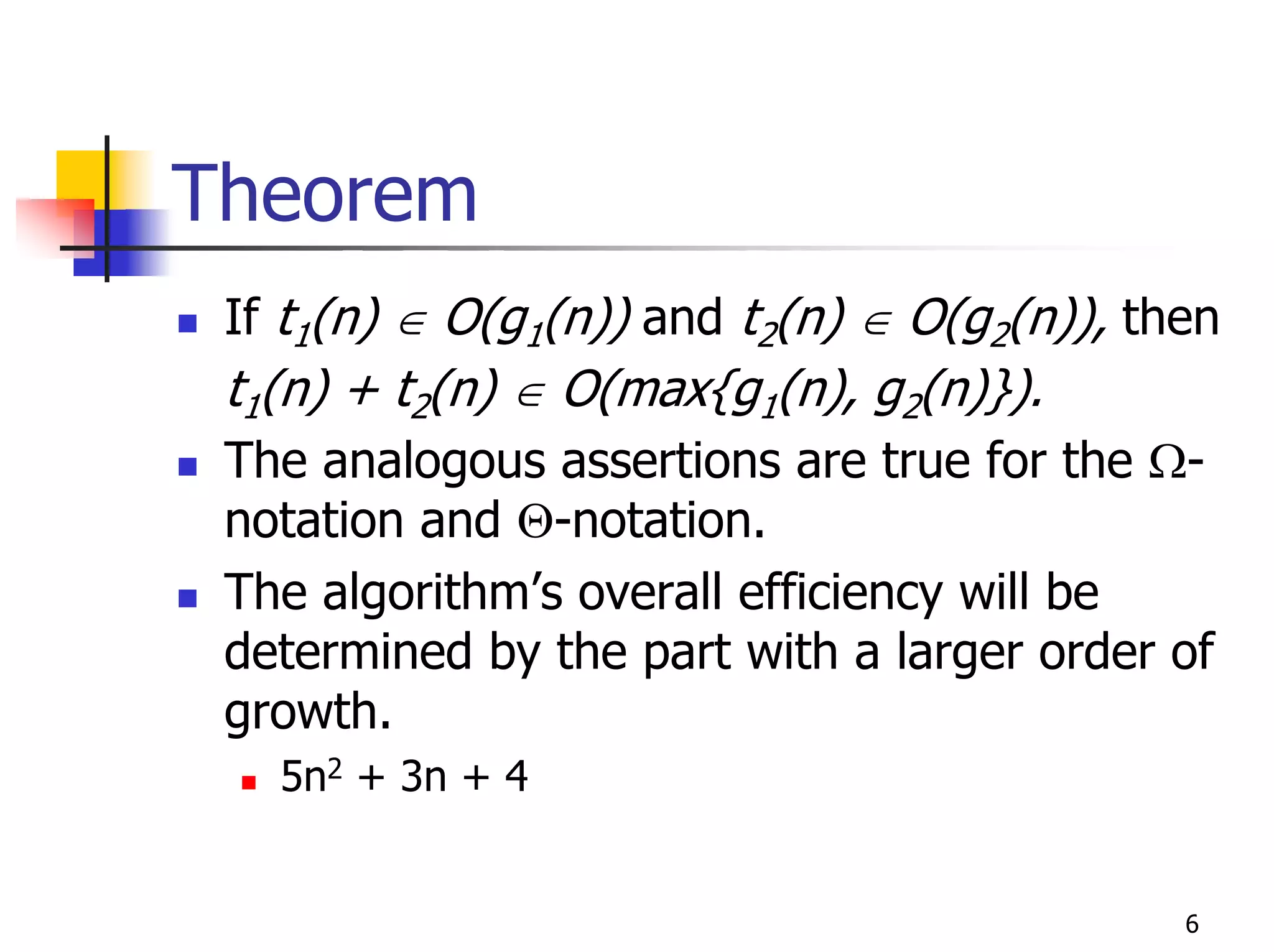
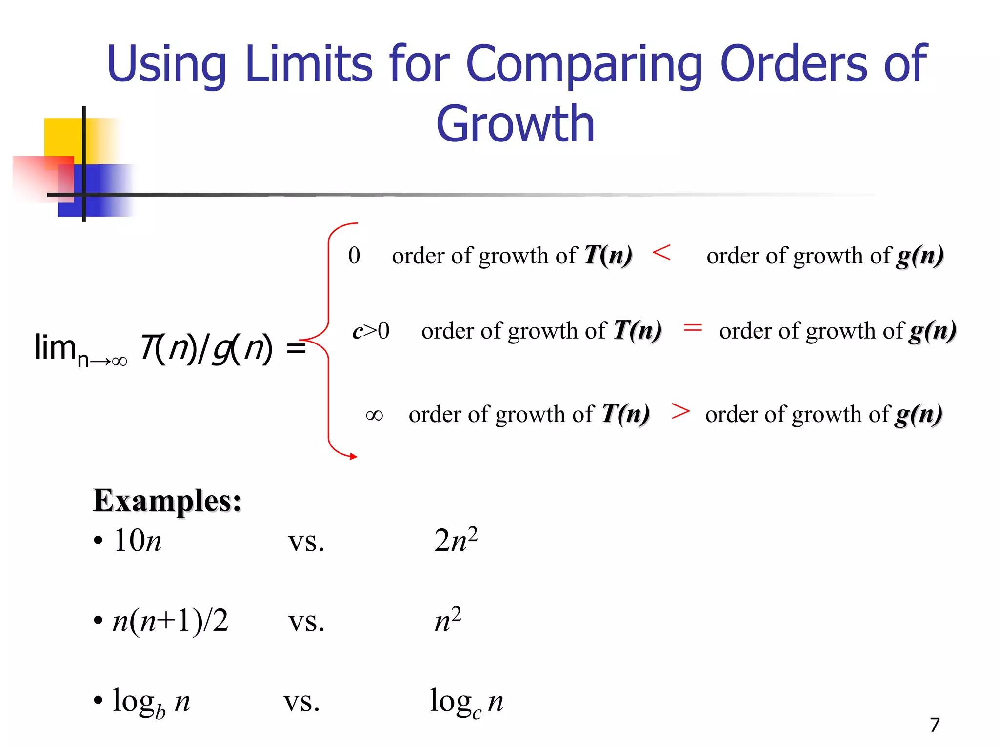
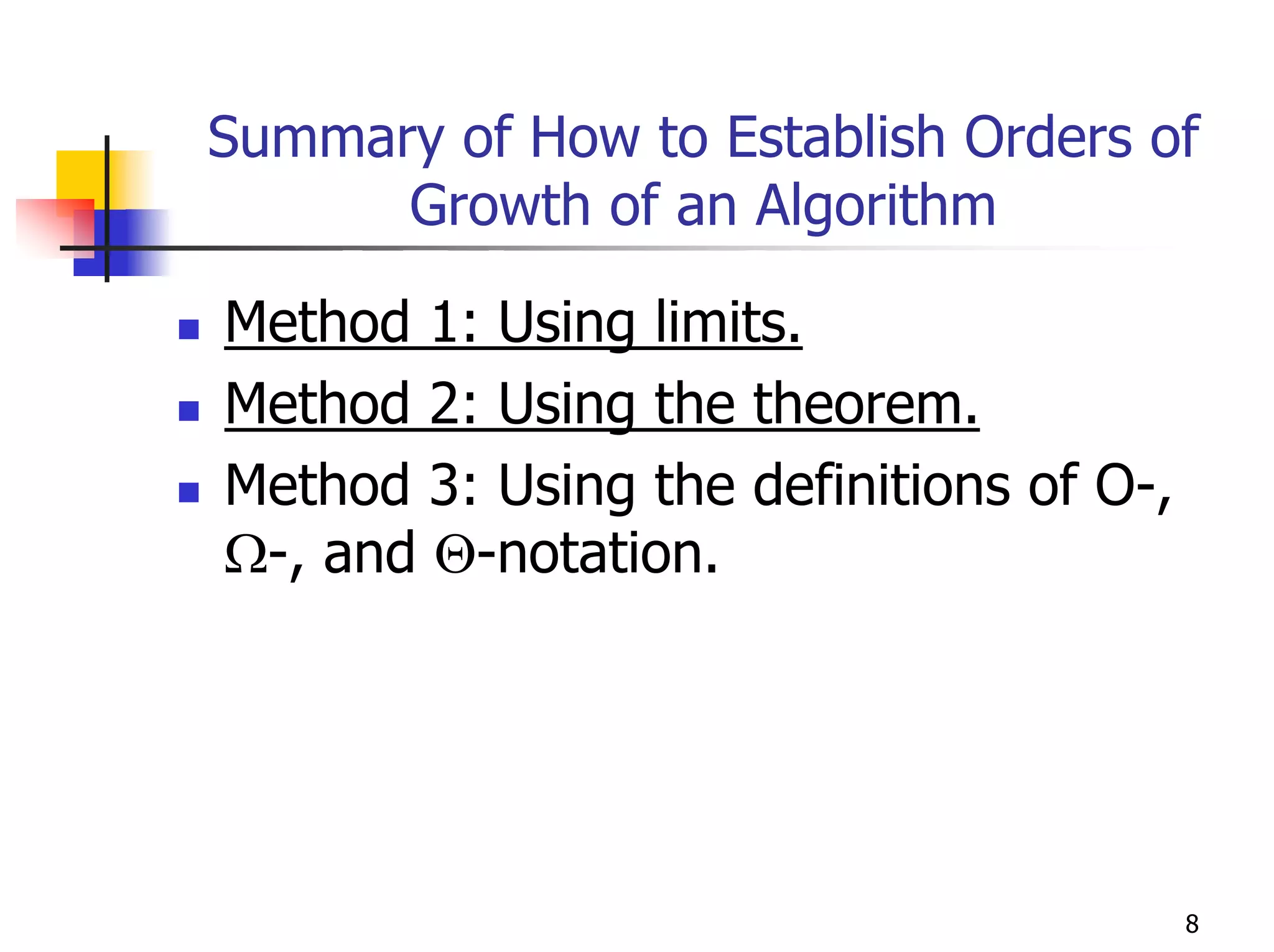
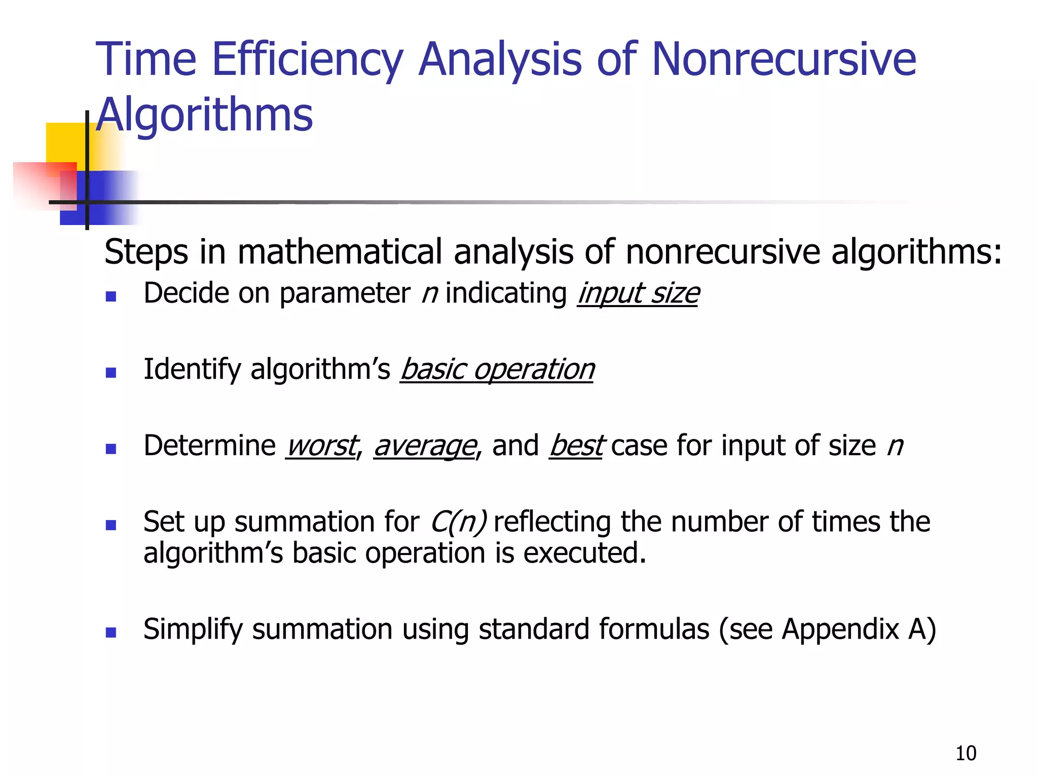
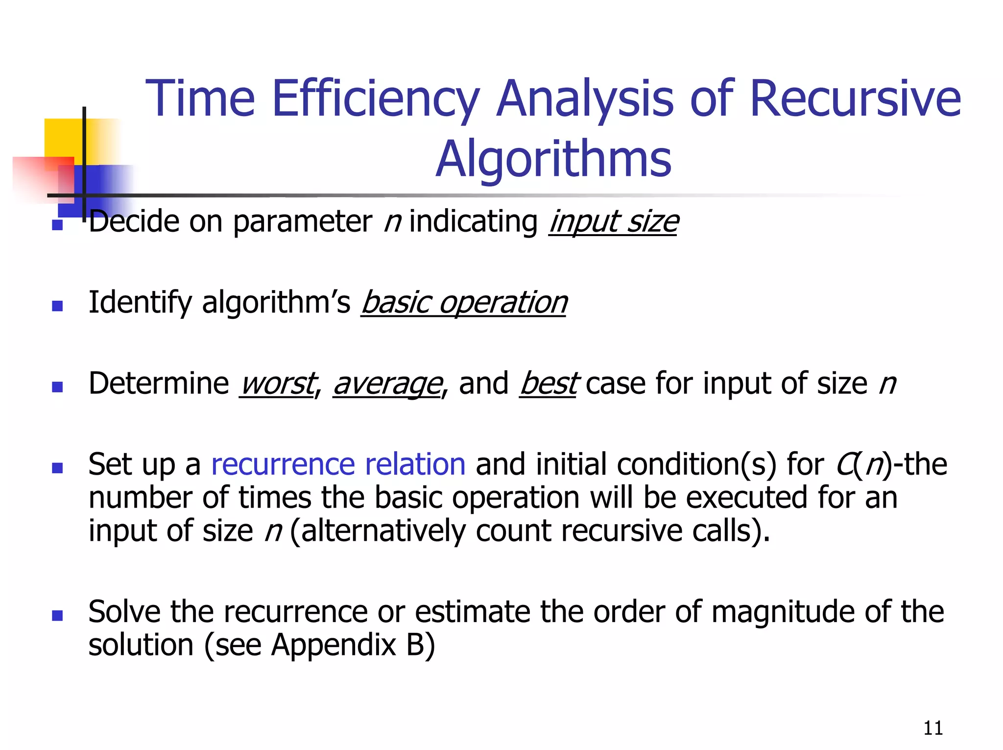
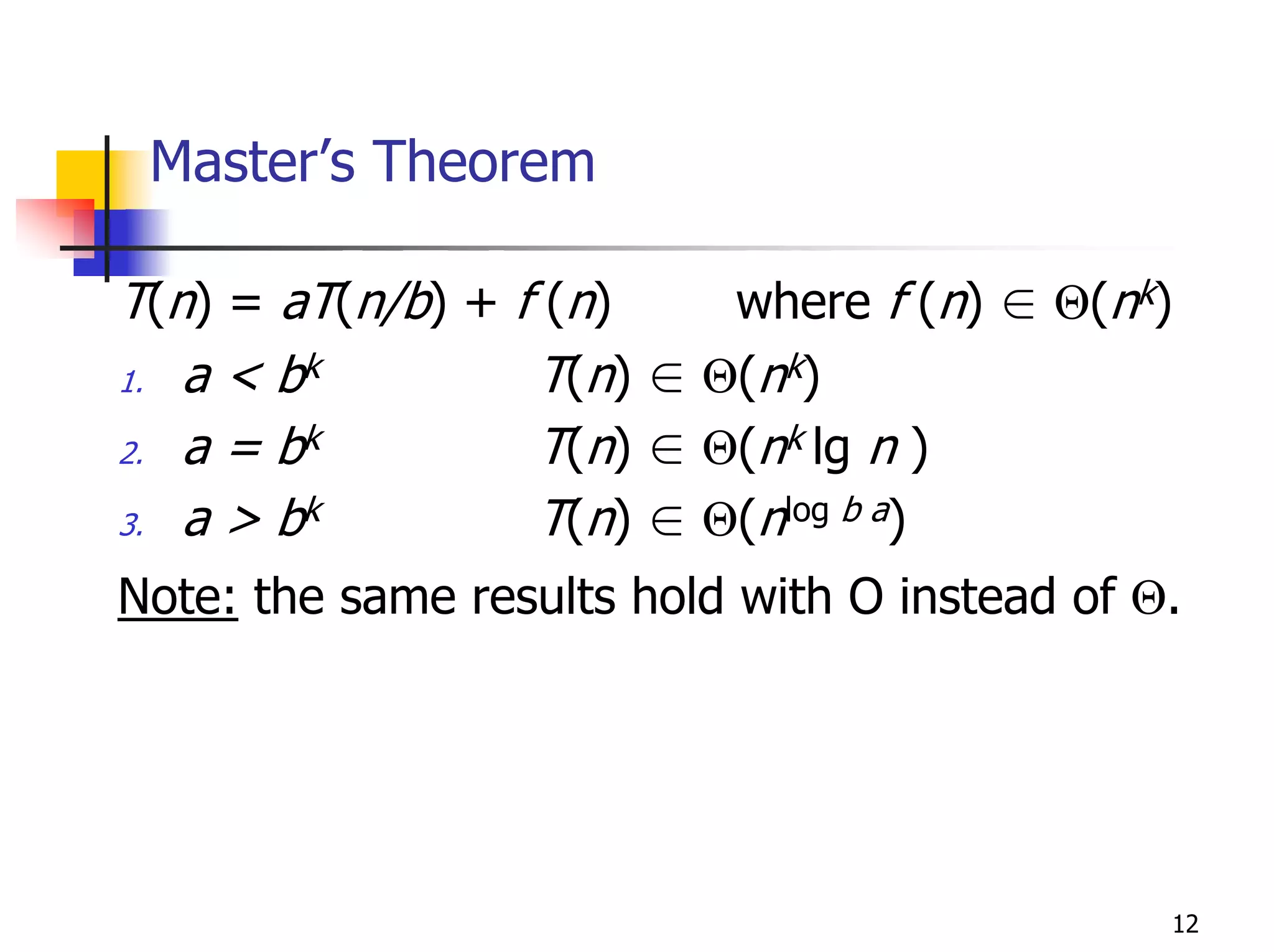
- Analyzing the time efficiency of recursive and non-recursive algorithms using orders of growth, recurrence relations, and the master's theorem.
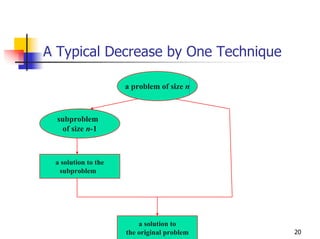
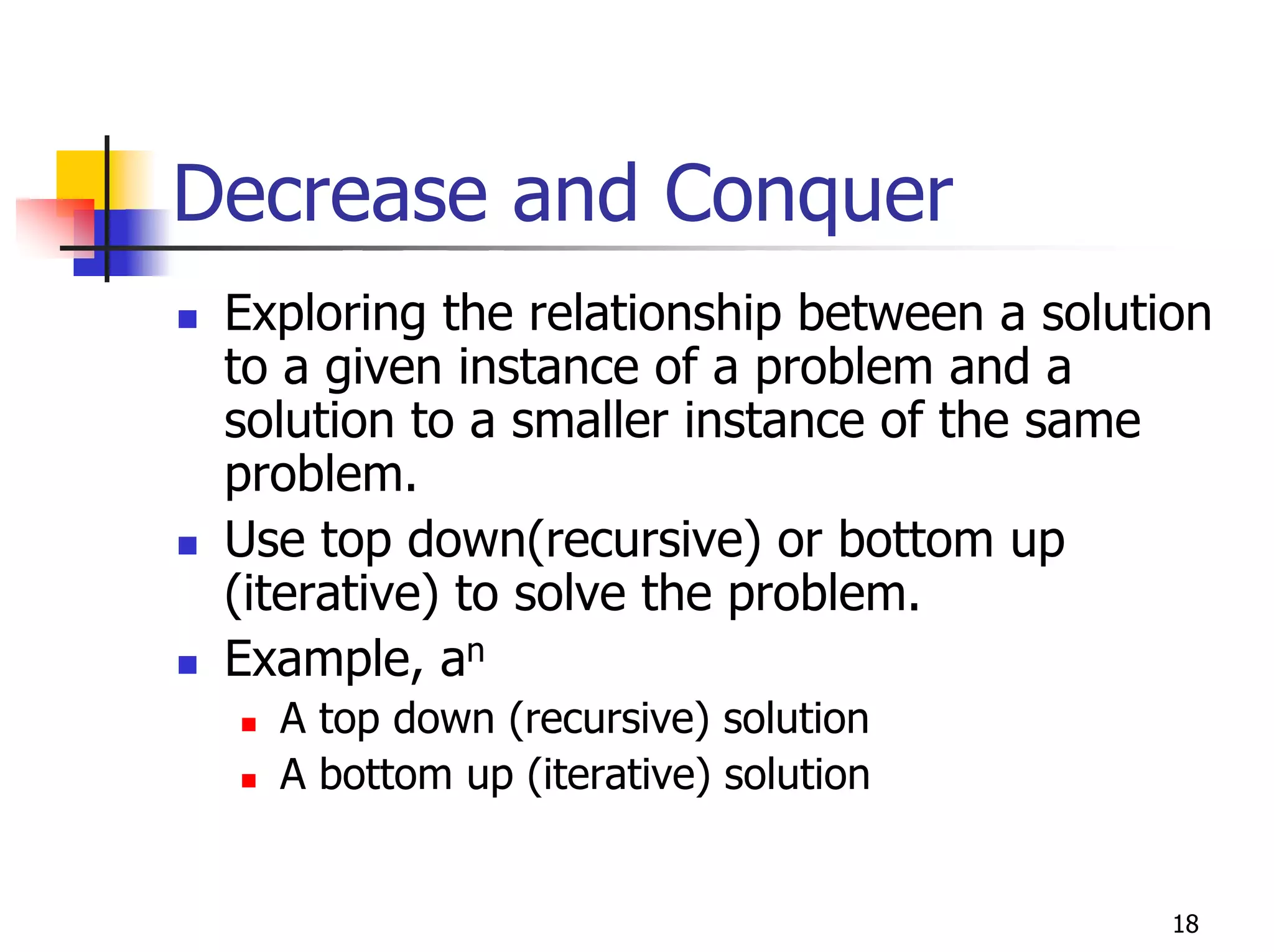
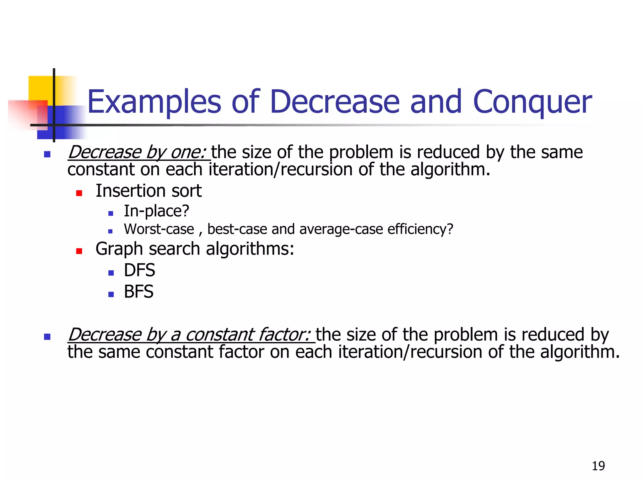
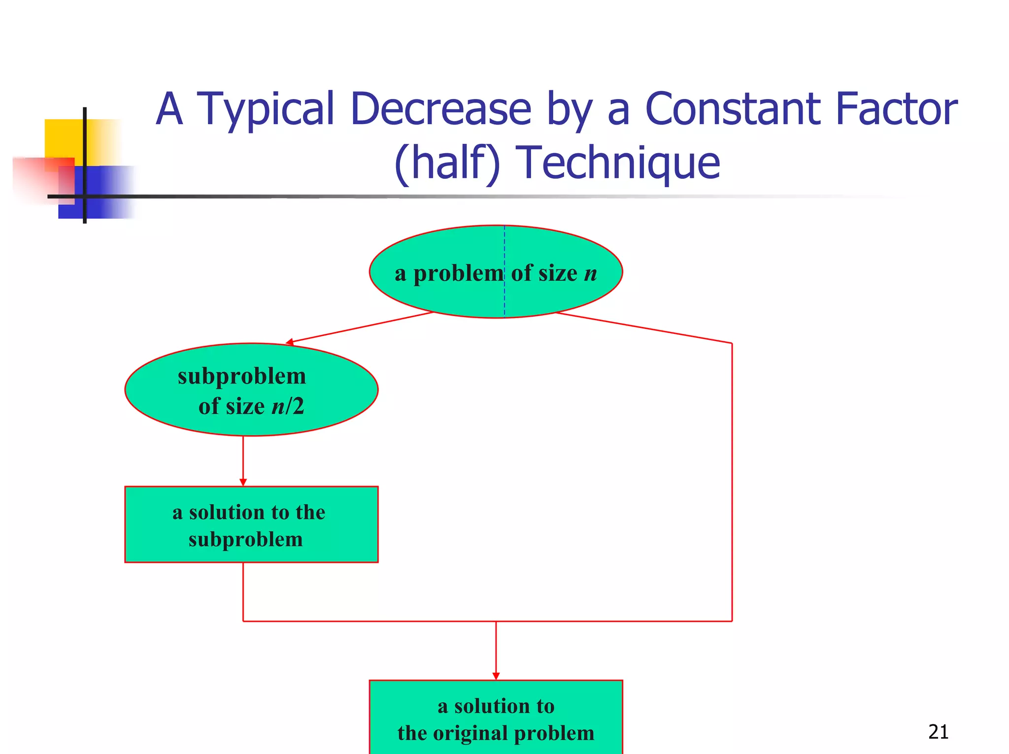
- Examples of specific algorithms that use techniques like divide-and-conquer, decrease-and-conquer, dynamic programming, and greedy strategies.
- Complexity classes like P, NP, and NP-complete problems.