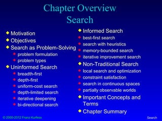
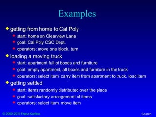
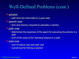
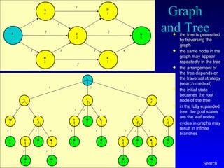
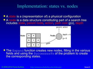
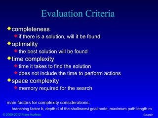
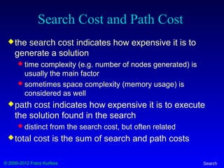
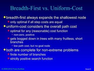
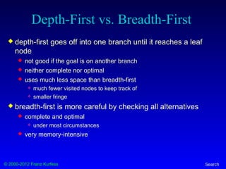
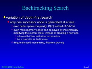
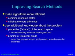
This document provides an overview of search techniques for problem solving. It discusses formulating problems as search tasks by defining states, operators, an initial state, and a goal test. It also covers uninformed search methods like breadth-first, depth-first, and iterative deepening, as well as informed search using heuristics. Example problems discussed include the vacuum world, 8-puzzle, 8-queens, and traveling salesman problem. State spaces and search graphs are used to represent problems formally.


![© 2000-2012 Franz Kurfess Search
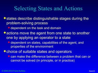
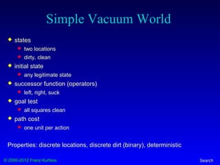
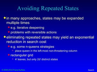
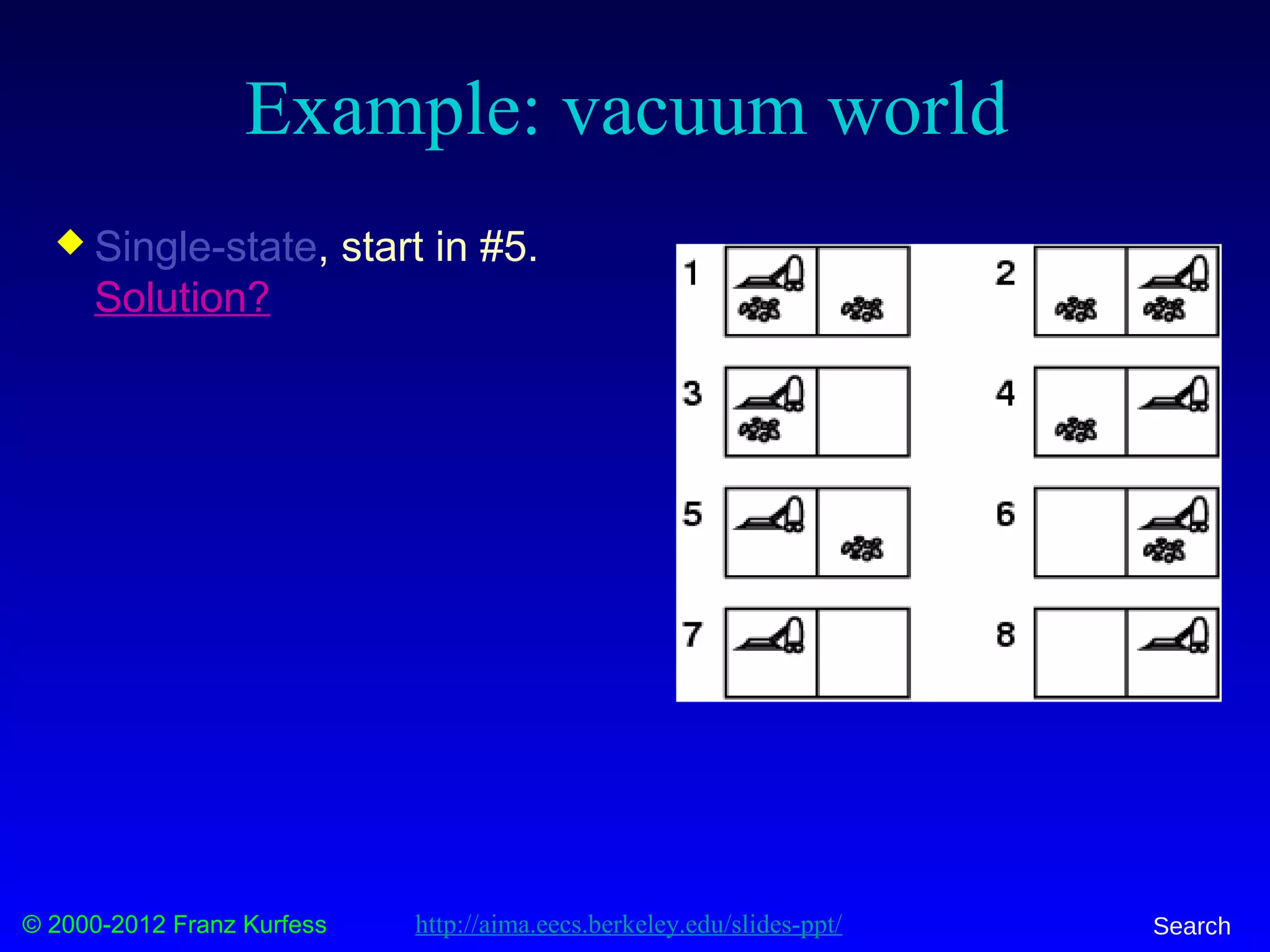
Example: vacuum world
Sensorless, start in
{1,2,3,4,5,6,7,8} e.g.,
Right goes to {2,4,6,8}
Solution?
[Right,Suck,Left,Suck]
Contingency
Nondeterministic: Suck may
dirty a clean carpet
Partially observable: location, dirt at current location.
Percept: [L, Clean], i.e., start in #5 or #7
Solution?
http://aima.eecs.berkeley.edu/slides-ppt/](https://image.slidesharecdn.com/3-search-160805142330/85/Artificial-Intelligence-Search-Algorithms-16-320.jpg)
![© 2000-2012 Franz Kurfess Search
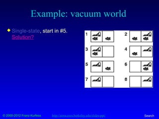
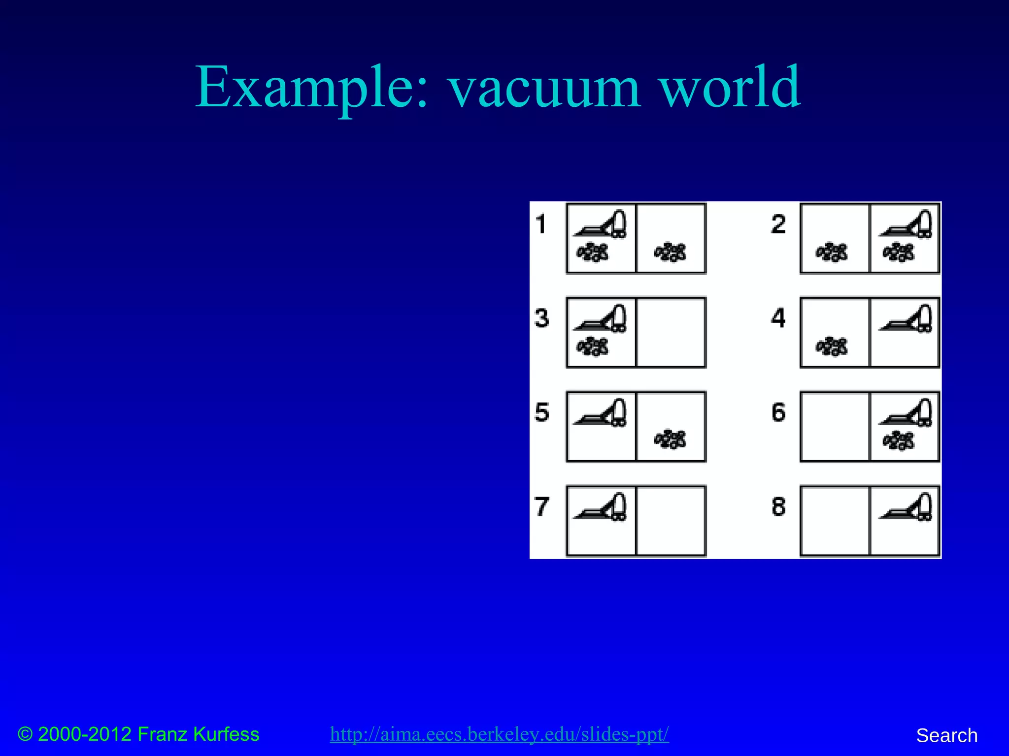
Example: vacuum world
Sensorless, start in
{1,2,3,4,5,6,7,8} e.g.,
Right goes to {2,4,6,8}
Solution?
[Right,Suck,Left,Suck]
Contingency
Nondeterministic: Suck may
dirty a clean carpet
Partially observable: location, dirt at current location.
Percept: [L, Clean], i.e., start in #5 or #7
Solution? [Right, if dirt then Suck]
http://aima.eecs.berkeley.edu/slides-ppt/](https://image.slidesharecdn.com/3-search-160805142330/85/Artificial-Intelligence-Search-Algorithms-17-320.jpg)
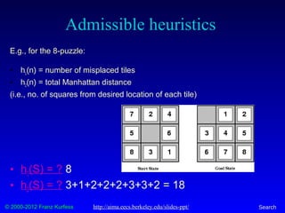
![© 2000-2012 Franz Kurfess Search
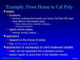
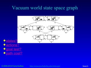
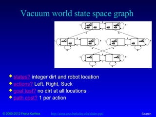
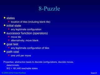
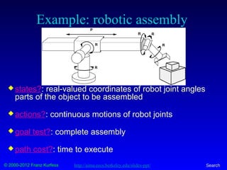
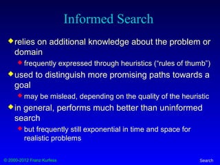
Example: The 8-puzzle
states?
actions?
goal test?
path cost?
[Note: optimal solution of n-Puzzle family is NP-hard]
http://aima.eecs.berkeley.edu/slides-ppt/](https://image.slidesharecdn.com/3-search-160805142330/85/Artificial-Intelligence-Search-Algorithms-22-320.jpg)


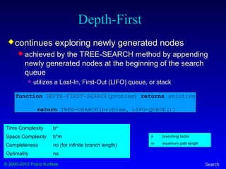
![© 2000-2012 Franz Kurfess Search
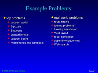
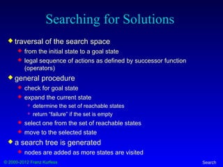
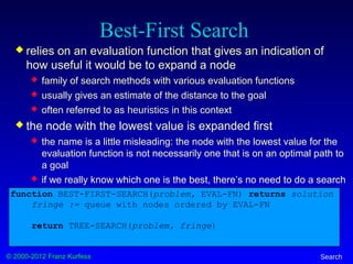
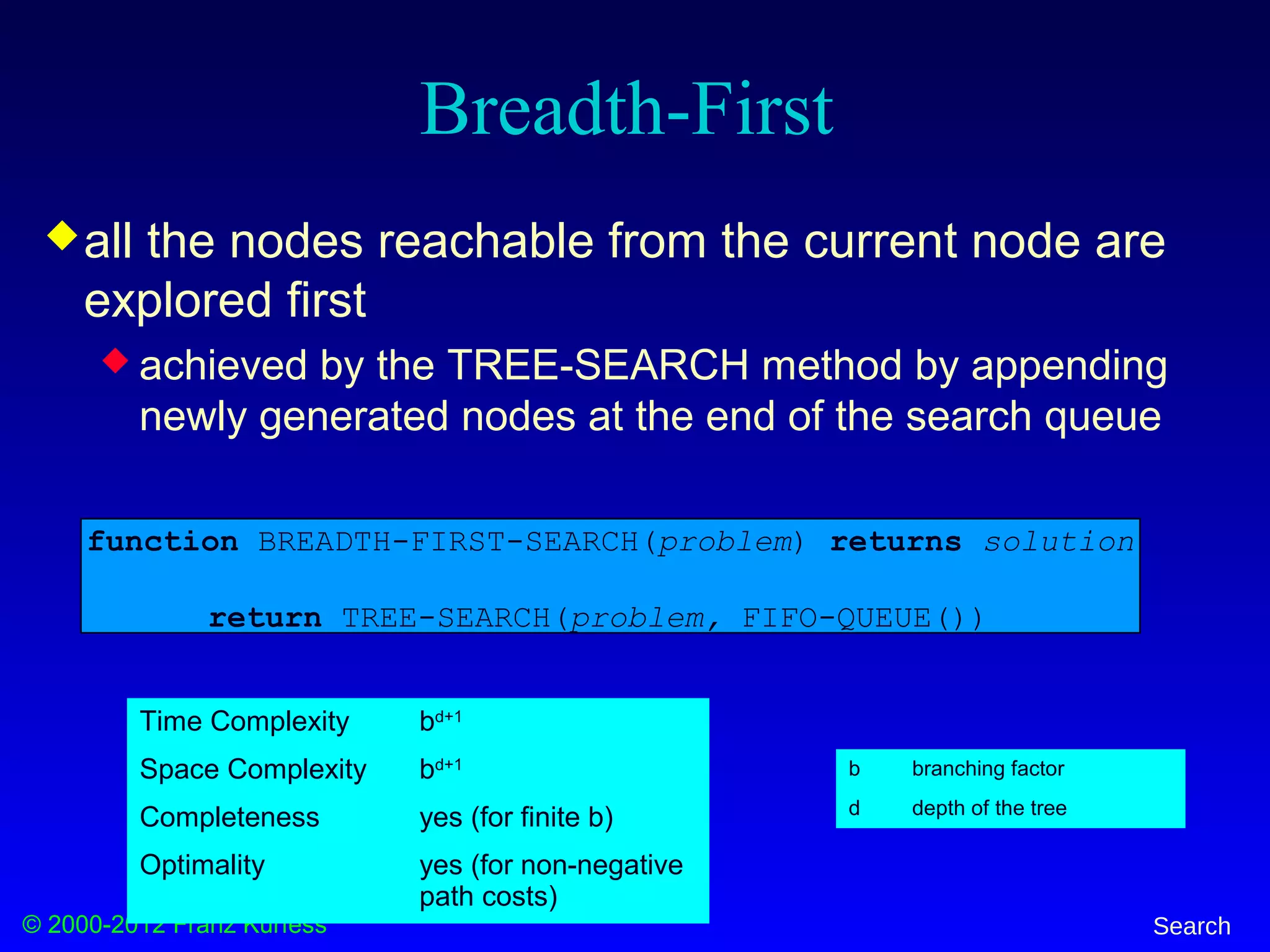
General Tree Search Algorithm
function TREE-SEARCH(problem, fringe) returns solution
fringe := INSERT(MAKE-NODE(INITIAL-STATE[problem]), fringe)
loop do
if EMPTY?(fringe) then return failure
node := REMOVE-FIRST(fringe)
if GOAL-TEST[problem] applied to STATE[node] succeeds
then return SOLUTION(node)
fringe := INSERT-ALL(EXPAND(node, problem), fringe)
generate the node from the initial state of the problem
repeat
return failure if there are no more nodes in the fringe
examine the current node; if it’s a goal, return the solution
expand the current node, and add the new nodes to the fringe
Note: This method is called “General-Search” in earlier AIMA editions](https://image.slidesharecdn.com/3-search-160805142330/85/Artificial-Intelligence-Search-Algorithms-40-320.jpg)
![© 2000-2012 Franz Kurfess Search
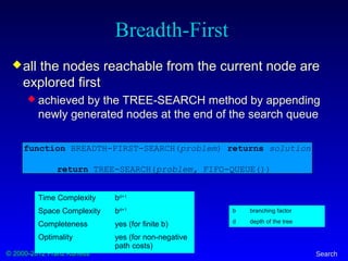
Breadth-First Snapshot 1
Initial
Visited
Fringe
Current
Visible
Goal
1
2 3
Fringe: [] + [2,3]](https://image.slidesharecdn.com/3-search-160805142330/85/Artificial-Intelligence-Search-Algorithms-47-320.jpg)
![© 2000-2012 Franz Kurfess Search
Breadth-First Snapshot 2
Initial
Visited
Fringe
Current
Visible
Goal
1
2 3
4 5
Fringe: [3] + [4,5]](https://image.slidesharecdn.com/3-search-160805142330/85/Artificial-Intelligence-Search-Algorithms-48-320.jpg)
![© 2000-2012 Franz Kurfess Search
Breadth-First Snapshot 3
Initial
Visited
Fringe
Current
Visible
Goal
1
2 3
4 5 6 7
Fringe: [4,5] + [6,7]](https://image.slidesharecdn.com/3-search-160805142330/85/Artificial-Intelligence-Search-Algorithms-49-320.jpg)
![© 2000-2012 Franz Kurfess Search
Breadth-First Snapshot 4
Initial
Visited
Fringe
Current
Visible
Goal
1
2 3
4 5 6 7
8 9
Fringe: [5,6,7] + [8,9]](https://image.slidesharecdn.com/3-search-160805142330/85/Artificial-Intelligence-Search-Algorithms-50-320.jpg)
![© 2000-2012 Franz Kurfess Search
Breadth-First Snapshot 5
Initial
Visited
Fringe
Current
Visible
Goal
1
2 3
4 5 6 7
8 9 10 11
Fringe: [6,7,8,9] + [10,11]](https://image.slidesharecdn.com/3-search-160805142330/85/Artificial-Intelligence-Search-Algorithms-51-320.jpg)
![© 2000-2012 Franz Kurfess Search
Breadth-First Snapshot 6
Initial
Visited
Fringe
Current
Visible
Goal
1
2 3
4 5 6 7
8 9 10 11 12 13
Fringe: [7,8,9,10,11] + [12,13]](https://image.slidesharecdn.com/3-search-160805142330/85/Artificial-Intelligence-Search-Algorithms-52-320.jpg)
![© 2000-2012 Franz Kurfess Search
Breadth-First Snapshot 7
Initial
Visited
Fringe
Current
Visible
Goal
1
2 3
4 5 6 7
8 9 10 11 12 13 14 15
Fringe: [8,9.10,11,12,13] + [14,15]](https://image.slidesharecdn.com/3-search-160805142330/85/Artificial-Intelligence-Search-Algorithms-53-320.jpg)
![© 2000-2012 Franz Kurfess Search
Breadth-First Snapshot 8
Initial
Visited
Fringe
Current
Visible
Goal
1
2 3
4 5 6 7
8 9 10 11 12 13 14 15
16 17
Fringe: [9,10,11,12,13,14,15] + [16,17]](https://image.slidesharecdn.com/3-search-160805142330/85/Artificial-Intelligence-Search-Algorithms-54-320.jpg)
![© 2000-2012 Franz Kurfess Search
Breadth-First Snapshot 9
Initial
Visited
Fringe
Current
Visible
Goal
1
2 3
4 5 6 7
8 9 10 11 12 13 14 15
16 17 18 19
Fringe: [10,11,12,13,14,15,16,17] + [18,19]](https://image.slidesharecdn.com/3-search-160805142330/85/Artificial-Intelligence-Search-Algorithms-55-320.jpg)
![© 2000-2012 Franz Kurfess Search
Breadth-First Snapshot 10
Initial
Visited
Fringe
Current
Visible
Goal
1
2 3
4 5 6 7
8 9 10 11 12 13 14 15
16 17 18 19 20 21
Fringe: [11,12,13,14,15,16,17,18,19] + [20,21]](https://image.slidesharecdn.com/3-search-160805142330/85/Artificial-Intelligence-Search-Algorithms-56-320.jpg)
![© 2000-2012 Franz Kurfess Search
Breadth-First Snapshot 11
Initial
Visited
Fringe
Current
Visible
Goal
1
2 3
4 5 6 7
8 9 10 11 12 13 14 15
16 17 18 19 20 21 22 23
Fringe: [12, 13, 14, 15, 16, 17, 18, 19, 20, 21] + [22,23]](https://image.slidesharecdn.com/3-search-160805142330/85/Artificial-Intelligence-Search-Algorithms-57-320.jpg)
![© 2000-2012 Franz Kurfess Search
Breadth-First Snapshot 12
Initial
Visited
Fringe
Current
Visible
Goal
1
2 3
4 5 6 7
8 9 10 11 12 13 14 15
16 17 18 19 20 21 22 23 24 25
Fringe: [13,14,15,16,17,18,19,20,21] + [22,23]
Note:
The goal node is
“visible” here,
but we can not
perform the goal
test yet.](https://image.slidesharecdn.com/3-search-160805142330/85/Artificial-Intelligence-Search-Algorithms-58-320.jpg)
![© 2000-2012 Franz Kurfess Search
Breadth-First Snapshot 13
Initial
Visited
Fringe
Current
Visible
Goal
1
2 3
4 5 6 7
8 9 10 11 12 13 14 15
16 17 18 19 20 21 22 23 24 25 26 27
Fringe: [14,15,16,17,18,19,20,21,22,23,24,25] + [26,27]](https://image.slidesharecdn.com/3-search-160805142330/85/Artificial-Intelligence-Search-Algorithms-59-320.jpg)
![© 2000-2012 Franz Kurfess Search
Breadth-First Snapshot 14
Initial
Visited
Fringe
Current
Visible
Goal
1
2 3
4 5 6 7
8 9 10 11 12 13 14 15
16 17 18 19 20 21 22 23 24 25 26 27 28 29
Fringe: [15,16,17,18,19,20,21,22,23,24,25,26,27] + [28,29]](https://image.slidesharecdn.com/3-search-160805142330/85/Artificial-Intelligence-Search-Algorithms-60-320.jpg)
![© 2000-2012 Franz Kurfess Search
Breadth-First Snapshot 15
Initial
Visited
Fringe
Current
Visible
Goal
1
2 3
4 5 6 7
8 9 10 11 12 13 14 15
16 17 18 19 20 21 22 23 24 25 26 27 28 29 30 31
Fringe: [15,16,17,18,19,20,21,22,23,24,25,26,27,28,29] + [30,31]](https://image.slidesharecdn.com/3-search-160805142330/85/Artificial-Intelligence-Search-Algorithms-61-320.jpg)
![© 2000-2012 Franz Kurfess Search
Breadth-First Snapshot 16
Initial
Visited
Fringe
Current
Visible
Goal
1
2 3
4 5 6 7
8 9 10 11 12 13 14 15
16 17 18 19 20 21 22 23 24 25 26 27 28 29 30 31
Fringe: [17,18,19,20,21,22,23,24,25,26,27,28,29,30,31]](https://image.slidesharecdn.com/3-search-160805142330/85/Artificial-Intelligence-Search-Algorithms-62-320.jpg)
![© 2000-2012 Franz Kurfess Search
Breadth-First Snapshot 17
Initial
Visited
Fringe
Current
Visible
Goal
1
2 3
4 5 6 7
8 9 10 11 12 13 14 15
16 17 18 19 20 21 22 23 24 25 26 27 28 29 30 31
Fringe: [18,19,20,21,22,23,24,25,26,27,28,29,30,31]](https://image.slidesharecdn.com/3-search-160805142330/85/Artificial-Intelligence-Search-Algorithms-63-320.jpg)
![© 2000-2012 Franz Kurfess Search
Breadth-First Snapshot 18
Initial
Visited
Fringe
Current
Visible
Goal
1
2 3
4 5 6 7
8 9 10 11 12 13 14 15
16 17 18 19 20 21 22 23 24 25 26 27 28 29 30 31
Fringe: [19,20,21,22,23,24,25,26,27,28,29,30,31]](https://image.slidesharecdn.com/3-search-160805142330/85/Artificial-Intelligence-Search-Algorithms-64-320.jpg)
![© 2000-2012 Franz Kurfess Search
Breadth-First Snapshot 19
Initial
Visited
Fringe
Current
Visible
Goal
1
2 3
4 5 6 7
8 9 10 11 12 13 14 15
16 17 18 19 20 21 22 23 24 25 26 27 28 29 30 31
Fringe: [20,21,22,23,24,25,26,27,28,29,30,31]](https://image.slidesharecdn.com/3-search-160805142330/85/Artificial-Intelligence-Search-Algorithms-65-320.jpg)
![© 2000-2012 Franz Kurfess Search
Breadth-First Snapshot 20
Initial
Visited
Fringe
Current
Visible
Goal
1
2 3
4 5 6 7
8 9 10 11 12 13 14 15
16 17 18 19 20 21 22 23 24 25 26 27 28 29 30 31
Fringe: [21,22,23,24,25,26,27,28,29,30,31]](https://image.slidesharecdn.com/3-search-160805142330/85/Artificial-Intelligence-Search-Algorithms-66-320.jpg)
![© 2000-2012 Franz Kurfess Search
Breadth-First Snapshot 21
Initial
Visited
Fringe
Current
Visible
Goal
1
2 3
4 5 6 7
8 9 10 11 12 13 14 15
16 17 18 19 20 21 22 23 24 25 26 27 28 29 30 31
Fringe: [22,23,24,25,26,27,28,29,30,31]](https://image.slidesharecdn.com/3-search-160805142330/85/Artificial-Intelligence-Search-Algorithms-67-320.jpg)
![© 2000-2012 Franz Kurfess Search
Breadth-First Snapshot 22
Initial
Visited
Fringe
Current
Visible
Goal
1
2 3
4 5 6 7
8 9 10 11 12 13 14 15
16 17 18 19 20 21 22 23 24 25 26 27 28 29 30 31
Fringe: [23,24,25,26,27,28,29,30,31]](https://image.slidesharecdn.com/3-search-160805142330/85/Artificial-Intelligence-Search-Algorithms-68-320.jpg)
![© 2000-2012 Franz Kurfess Search
Breadth-First Snapshot 23
Initial
Visited
Fringe
Current
Visible
Goal
1
2 3
4 5 6 7
8 9 10 11 12 13 14 15
16 17 18 19 20 21 22 23 24 25 26 27 28 29 30 31
Fringe: [24,25,26,27,28,29,30,31]](https://image.slidesharecdn.com/3-search-160805142330/85/Artificial-Intelligence-Search-Algorithms-69-320.jpg)
![© 2000-2012 Franz Kurfess Search
Breadth-First Snapshot 24
Initial
Visited
Fringe
Current
Visible
Goal
1
2 3
4 5 6 7
8 9 10 11 12 13 14 15
16 17 18 19 20 21 22 23 24 25 26 27 28 29 30 31
Fringe: [25,26,27,28,29,30,31]
Note:
The goal test is
positive for this
node, and a
solution is found
in 24 steps.](https://image.slidesharecdn.com/3-search-160805142330/85/Artificial-Intelligence-Search-Algorithms-70-320.jpg)
![© 2000-2012 Franz Kurfess Search
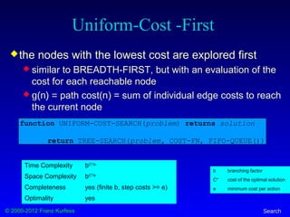
Uniform-Cost Snapshot
Initial
Visited
Fringe
Current
Visible
Goal
1
2 3
4 5 6 7
8 9 10 11 12 13 14 15
16 17 18 19 20 21 22 23 24 25 26 27 28 29 30 31
4 3
7
2
2 2 4
5 4 4 4 3 6 9
3 4 7 2 4 8 6 4 3 4 2 3 9 25 8
Fringe: [27(10), 4(11), 25(12), 26(12), 14(13), 24(13), 20(14), 15(16), 21(18)]
+ [22(16), 23(15)]
Edge Cost 9](https://image.slidesharecdn.com/3-search-160805142330/85/Artificial-Intelligence-Search-Algorithms-72-320.jpg)
![© 2000-2012 Franz Kurfess Search
Uniform Cost Fringe Trace
1. [1(0)]
2. [3(3), 2(4)]
3. [2(4), 6(5), 7(7)]
4. [6(5), 5(6), 7(7), 4(11)]
5. [5(6), 7(7), 13(8), 12(9), 4(11)]
6. [7(7), 13(8), 12(9), 10(10), 11(10), 4(11)]
7. [13(8), 12(9), 10(10), 11(10), 4(11), 14(13), 15(16)]
8. [12(9), 10(10), 11(10), 27(10), 4(11), 26(12), 14(13), 15(16)]
9. [10(10), 11(10), 27(10), 4(11), 26(12), 25(12), 14(13), 24(13), 15(16)]
10. [11(10), 27(10), 4(11), 25(12), 26(12), 14(13), 24(13), 20(14), 15(16), 21(18)]
11. [27(10), 4(11), 25(12), 26(12), 14(13), 24(13), 20(14), 23(15), 15(16), 22(16), 21(18)]
12. [4(11), 25(12), 26(12), 14(13), 24(13), 20(14), 23(15), 15(16), 23(16), 21(18)]
13. [25(12), 26(12), 14(13), 24(13),8(13), 20(14), 23(15), 15(16), 23(16), 9(16), 21(18)]
14. [26(12), 14(13), 24(13),8(13), 20(14), 23(15), 15(16), 23(16), 9(16), 21(18)]
15. [14(13), 24(13),8(13), 20(14), 23(15), 15(16), 23(16), 9(16), 21(18)]
16. [24(13),8(13), 20(14), 23(15), 15(16), 23(16), 9(16), 29(16),21(18), 28(21)]
Goal reached!
Notation: [Bold+Yellow: Current Node; White: Old Fringe Node; Green+Italics: New Fringe Node].
Assumption: New nodes with the same cost as existing nodes are added after the existing node.](https://image.slidesharecdn.com/3-search-160805142330/85/Artificial-Intelligence-Search-Algorithms-73-320.jpg)
![© 2000-2012 Franz Kurfess Search
Depth-First Snapshot
Initial
Visited
Fringe
Current
Visible
Goal
1
2 3
4 5 6 7
8 9 10 11 12 13 14 15
16 17 18 19 20 21 22 23 24 25 26 27 28 29 30 31
Fringe: [3] + [22,23]](https://image.slidesharecdn.com/3-search-160805142330/85/Artificial-Intelligence-Search-Algorithms-76-320.jpg)

![© 2000-2012 Franz Kurfess Search
Greedy Best-First Search Snapshot
77 6 5 4 3 2 1 0 1 3 5 62 48
65 4 2 4 537
65 56
77
9 Initial
Visited
Fringe
Current
Visible
Goal
1
2 3
4 5 6 7
8 9 10 11 12 13 14 15
16 17 18 19 20 21 22 23 24 25 26 27 28 29 30 31
Fringe: [13(4), 7(6), 8(7)] + [24(0), 25(1)]
7Heuristics](https://image.slidesharecdn.com/3-search-160805142330/85/Artificial-Intelligence-Search-Algorithms-92-320.jpg)
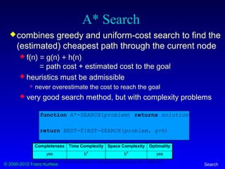
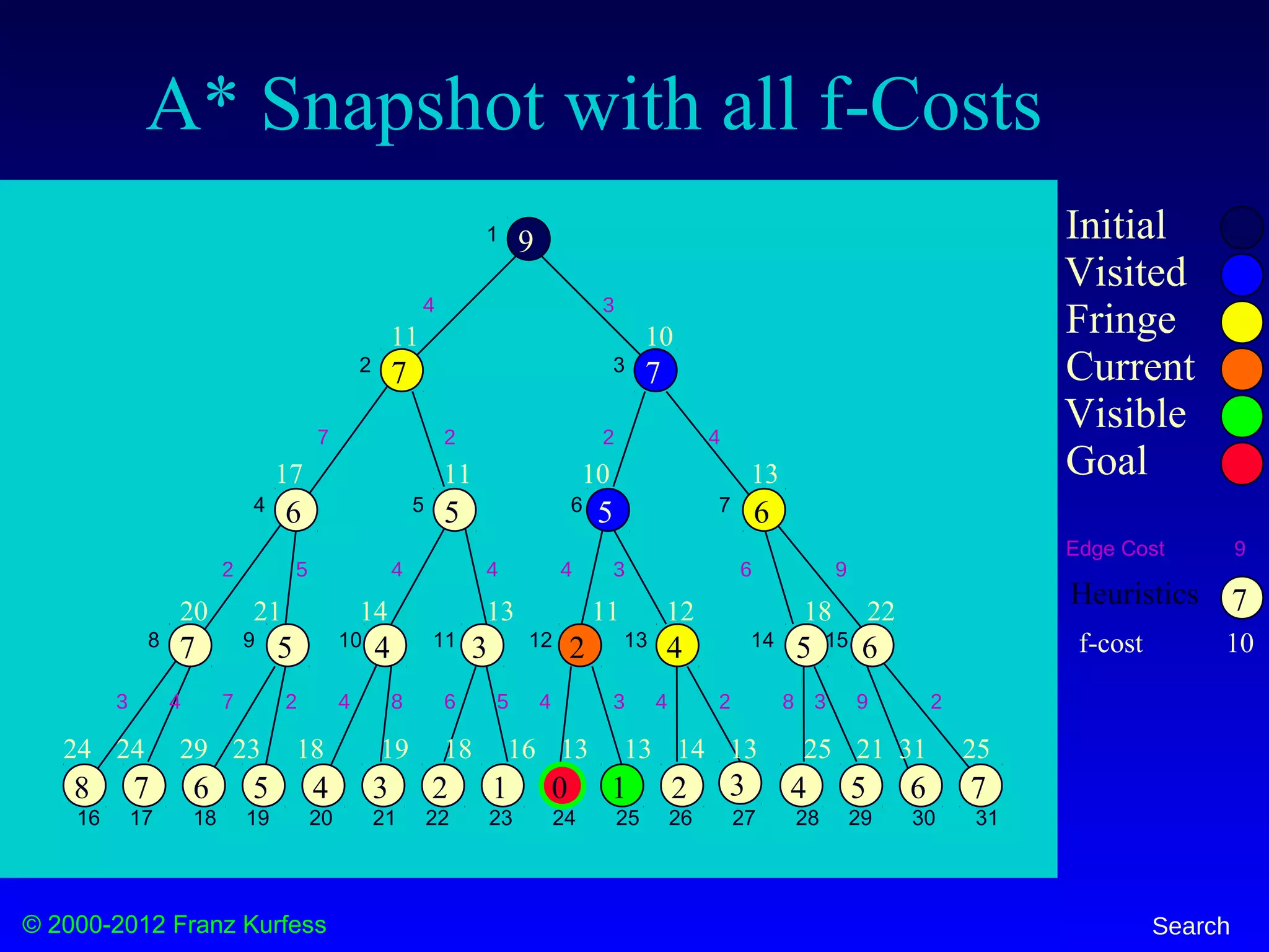
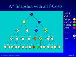
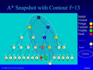
![© 2000-2012 Franz Kurfess Search
A* Snapshot
77 6 5 4 3 2 1 0 1 3 5 62 48
65 4 2 4 537
65 56
77
9 Initial
Visited
Fringe
Current
Visible
Goal
1
2 3
4 5 6 7
8 9 10 11 12 13 14 15
16 17 18 19 20 21 22 23 24 25 26 27 28 29 30 31
4 3
7
2
2 2 4
5 4 4 4 3 6 9
3 4 7 2 4 8 6 4 3 4 2 3 9 25 8
Fringe: [2(4+7), 13(3+2+3+4), 7(3+4+6)] + [24(3+2+4+4+0), 25(3+2+4+3+1)]
Edge Cost
7Heuristics
9
f-cost 10
9
11 10
11
10 13
12
13 13](https://image.slidesharecdn.com/3-search-160805142330/85/Artificial-Intelligence-Search-Algorithms-94-320.jpg)


![© 2000-2012 Franz Kurfess Search
Example: vacuum world
Sensorless, start in
{1,2,3,4,5,6,7,8} e.g.,
Right goes to {2,4,6,8}
Solution?
[Right,Suck,Left,Suck]
Contingency
Nondeterministic: Suck may
dirty a clean carpet
Partially observable: location, dirt at current location.
Percept: [L, Clean], i.e., start in #5 or #7
Solution?
http://aima.eecs.berkeley.edu/slides-ppt/](https://image.slidesharecdn.com/3-search-160805142330/75/Artificial-Intelligence-Search-Algorithms-16-2048.jpg)
![© 2000-2012 Franz Kurfess Search
Example: vacuum world
Sensorless, start in
{1,2,3,4,5,6,7,8} e.g.,
Right goes to {2,4,6,8}
Solution?
[Right,Suck,Left,Suck]
Contingency
Nondeterministic: Suck may
dirty a clean carpet
Partially observable: location, dirt at current location.
Percept: [L, Clean], i.e., start in #5 or #7
Solution? [Right, if dirt then Suck]
http://aima.eecs.berkeley.edu/slides-ppt/](https://image.slidesharecdn.com/3-search-160805142330/75/Artificial-Intelligence-Search-Algorithms-17-2048.jpg)


![© 2000-2012 Franz Kurfess Search
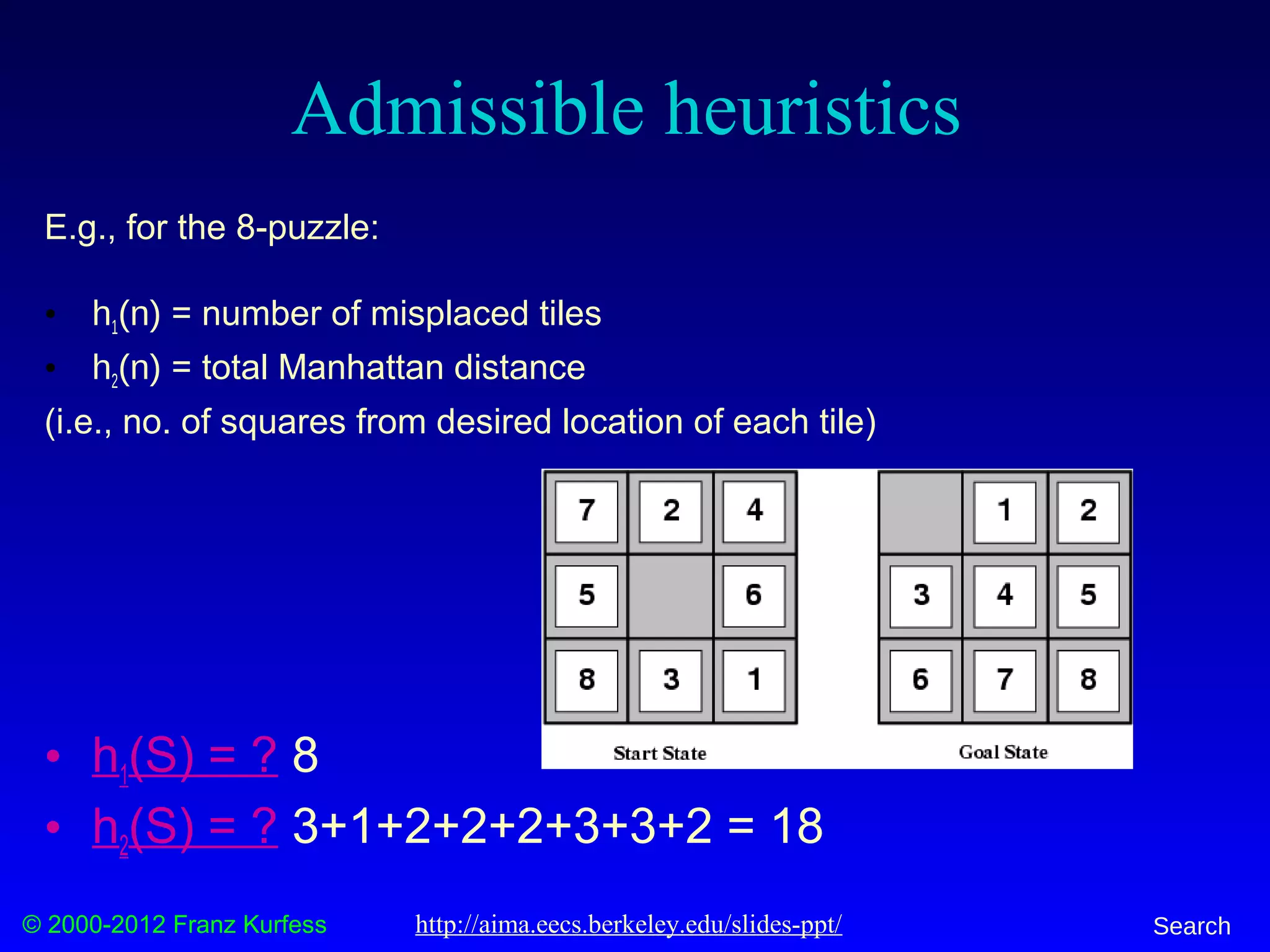
Example: The 8-puzzle
states?
actions?
goal test?
path cost?
[Note: optimal solution of n-Puzzle family is NP-hard]
http://aima.eecs.berkeley.edu/slides-ppt/](https://image.slidesharecdn.com/3-search-160805142330/75/Artificial-Intelligence-Search-Algorithms-22-2048.jpg)


![© 2000-2012 Franz Kurfess Search
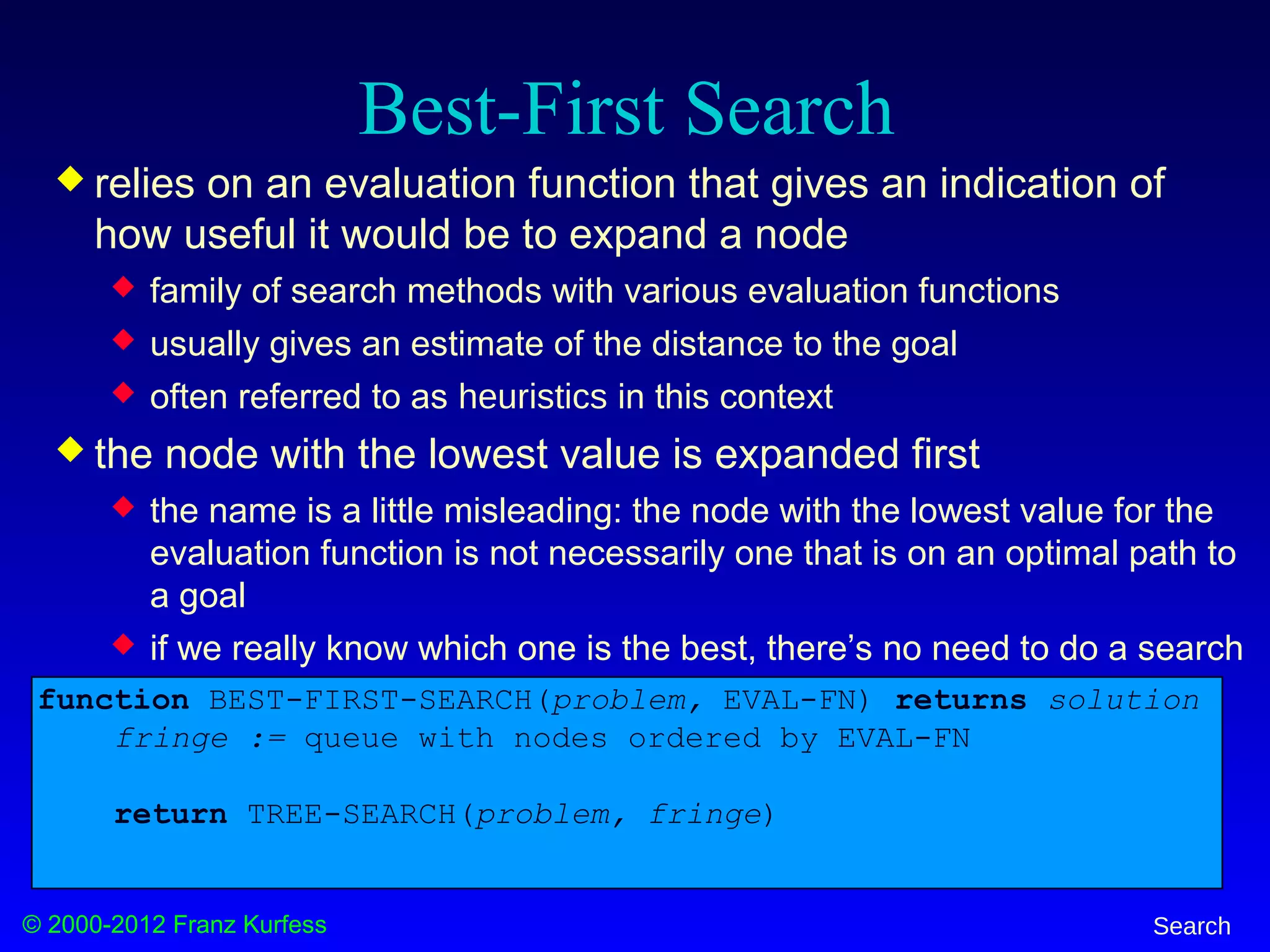
General Tree Search Algorithm
function TREE-SEARCH(problem, fringe) returns solution
fringe := INSERT(MAKE-NODE(INITIAL-STATE[problem]), fringe)
loop do
if EMPTY?(fringe) then return failure
node := REMOVE-FIRST(fringe)
if GOAL-TEST[problem] applied to STATE[node] succeeds
then return SOLUTION(node)
fringe := INSERT-ALL(EXPAND(node, problem), fringe)
generate the node from the initial state of the problem
repeat
return failure if there are no more nodes in the fringe
examine the current node; if it’s a goal, return the solution
expand the current node, and add the new nodes to the fringe
Note: This method is called “General-Search” in earlier AIMA editions](https://image.slidesharecdn.com/3-search-160805142330/75/Artificial-Intelligence-Search-Algorithms-40-2048.jpg)

![© 2000-2012 Franz Kurfess Search
Breadth-First Snapshot 1
Initial
Visited
Fringe
Current
Visible
Goal
1
2 3
Fringe: [] + [2,3]](https://image.slidesharecdn.com/3-search-160805142330/75/Artificial-Intelligence-Search-Algorithms-47-2048.jpg)
![© 2000-2012 Franz Kurfess Search
Breadth-First Snapshot 2
Initial
Visited
Fringe
Current
Visible
Goal
1
2 3
4 5
Fringe: [3] + [4,5]](https://image.slidesharecdn.com/3-search-160805142330/75/Artificial-Intelligence-Search-Algorithms-48-2048.jpg)
![© 2000-2012 Franz Kurfess Search
Breadth-First Snapshot 3
Initial
Visited
Fringe
Current
Visible
Goal
1
2 3
4 5 6 7
Fringe: [4,5] + [6,7]](https://image.slidesharecdn.com/3-search-160805142330/75/Artificial-Intelligence-Search-Algorithms-49-2048.jpg)
![© 2000-2012 Franz Kurfess Search
Breadth-First Snapshot 4
Initial
Visited
Fringe
Current
Visible
Goal
1
2 3
4 5 6 7
8 9
Fringe: [5,6,7] + [8,9]](https://image.slidesharecdn.com/3-search-160805142330/75/Artificial-Intelligence-Search-Algorithms-50-2048.jpg)
![© 2000-2012 Franz Kurfess Search
Breadth-First Snapshot 5
Initial
Visited
Fringe
Current
Visible
Goal
1
2 3
4 5 6 7
8 9 10 11
Fringe: [6,7,8,9] + [10,11]](https://image.slidesharecdn.com/3-search-160805142330/75/Artificial-Intelligence-Search-Algorithms-51-2048.jpg)
![© 2000-2012 Franz Kurfess Search
Breadth-First Snapshot 6
Initial
Visited
Fringe
Current
Visible
Goal
1
2 3
4 5 6 7
8 9 10 11 12 13
Fringe: [7,8,9,10,11] + [12,13]](https://image.slidesharecdn.com/3-search-160805142330/75/Artificial-Intelligence-Search-Algorithms-52-2048.jpg)
![© 2000-2012 Franz Kurfess Search
Breadth-First Snapshot 7
Initial
Visited
Fringe
Current
Visible
Goal
1
2 3
4 5 6 7
8 9 10 11 12 13 14 15
Fringe: [8,9.10,11,12,13] + [14,15]](https://image.slidesharecdn.com/3-search-160805142330/75/Artificial-Intelligence-Search-Algorithms-53-2048.jpg)
![© 2000-2012 Franz Kurfess Search
Breadth-First Snapshot 8
Initial
Visited
Fringe
Current
Visible
Goal
1
2 3
4 5 6 7
8 9 10 11 12 13 14 15
16 17
Fringe: [9,10,11,12,13,14,15] + [16,17]](https://image.slidesharecdn.com/3-search-160805142330/75/Artificial-Intelligence-Search-Algorithms-54-2048.jpg)
![© 2000-2012 Franz Kurfess Search
Breadth-First Snapshot 9
Initial
Visited
Fringe
Current
Visible
Goal
1
2 3
4 5 6 7
8 9 10 11 12 13 14 15
16 17 18 19
Fringe: [10,11,12,13,14,15,16,17] + [18,19]](https://image.slidesharecdn.com/3-search-160805142330/75/Artificial-Intelligence-Search-Algorithms-55-2048.jpg)
![© 2000-2012 Franz Kurfess Search
Breadth-First Snapshot 10
Initial
Visited
Fringe
Current
Visible
Goal
1
2 3
4 5 6 7
8 9 10 11 12 13 14 15
16 17 18 19 20 21
Fringe: [11,12,13,14,15,16,17,18,19] + [20,21]](https://image.slidesharecdn.com/3-search-160805142330/75/Artificial-Intelligence-Search-Algorithms-56-2048.jpg)
![© 2000-2012 Franz Kurfess Search
Breadth-First Snapshot 11
Initial
Visited
Fringe
Current
Visible
Goal
1
2 3
4 5 6 7
8 9 10 11 12 13 14 15
16 17 18 19 20 21 22 23
Fringe: [12, 13, 14, 15, 16, 17, 18, 19, 20, 21] + [22,23]](https://image.slidesharecdn.com/3-search-160805142330/75/Artificial-Intelligence-Search-Algorithms-57-2048.jpg)
![© 2000-2012 Franz Kurfess Search
Breadth-First Snapshot 12
Initial
Visited
Fringe
Current
Visible
Goal
1
2 3
4 5 6 7
8 9 10 11 12 13 14 15
16 17 18 19 20 21 22 23 24 25
Fringe: [13,14,15,16,17,18,19,20,21] + [22,23]
Note:
The goal node is
“visible” here,
but we can not
perform the goal
test yet.](https://image.slidesharecdn.com/3-search-160805142330/75/Artificial-Intelligence-Search-Algorithms-58-2048.jpg)
![© 2000-2012 Franz Kurfess Search
Breadth-First Snapshot 13
Initial
Visited
Fringe
Current
Visible
Goal
1
2 3
4 5 6 7
8 9 10 11 12 13 14 15
16 17 18 19 20 21 22 23 24 25 26 27
Fringe: [14,15,16,17,18,19,20,21,22,23,24,25] + [26,27]](https://image.slidesharecdn.com/3-search-160805142330/75/Artificial-Intelligence-Search-Algorithms-59-2048.jpg)
![© 2000-2012 Franz Kurfess Search
Breadth-First Snapshot 14
Initial
Visited
Fringe
Current
Visible
Goal
1
2 3
4 5 6 7
8 9 10 11 12 13 14 15
16 17 18 19 20 21 22 23 24 25 26 27 28 29
Fringe: [15,16,17,18,19,20,21,22,23,24,25,26,27] + [28,29]](https://image.slidesharecdn.com/3-search-160805142330/75/Artificial-Intelligence-Search-Algorithms-60-2048.jpg)
![© 2000-2012 Franz Kurfess Search
Breadth-First Snapshot 15
Initial
Visited
Fringe
Current
Visible
Goal
1
2 3
4 5 6 7
8 9 10 11 12 13 14 15
16 17 18 19 20 21 22 23 24 25 26 27 28 29 30 31
Fringe: [15,16,17,18,19,20,21,22,23,24,25,26,27,28,29] + [30,31]](https://image.slidesharecdn.com/3-search-160805142330/75/Artificial-Intelligence-Search-Algorithms-61-2048.jpg)
![© 2000-2012 Franz Kurfess Search
Breadth-First Snapshot 16
Initial
Visited
Fringe
Current
Visible
Goal
1
2 3
4 5 6 7
8 9 10 11 12 13 14 15
16 17 18 19 20 21 22 23 24 25 26 27 28 29 30 31
Fringe: [17,18,19,20,21,22,23,24,25,26,27,28,29,30,31]](https://image.slidesharecdn.com/3-search-160805142330/75/Artificial-Intelligence-Search-Algorithms-62-2048.jpg)
![© 2000-2012 Franz Kurfess Search
Breadth-First Snapshot 17
Initial
Visited
Fringe
Current
Visible
Goal
1
2 3
4 5 6 7
8 9 10 11 12 13 14 15
16 17 18 19 20 21 22 23 24 25 26 27 28 29 30 31
Fringe: [18,19,20,21,22,23,24,25,26,27,28,29,30,31]](https://image.slidesharecdn.com/3-search-160805142330/75/Artificial-Intelligence-Search-Algorithms-63-2048.jpg)
![© 2000-2012 Franz Kurfess Search
Breadth-First Snapshot 18
Initial
Visited
Fringe
Current
Visible
Goal
1
2 3
4 5 6 7
8 9 10 11 12 13 14 15
16 17 18 19 20 21 22 23 24 25 26 27 28 29 30 31
Fringe: [19,20,21,22,23,24,25,26,27,28,29,30,31]](https://image.slidesharecdn.com/3-search-160805142330/75/Artificial-Intelligence-Search-Algorithms-64-2048.jpg)
![© 2000-2012 Franz Kurfess Search
Breadth-First Snapshot 19
Initial
Visited
Fringe
Current
Visible
Goal
1
2 3
4 5 6 7
8 9 10 11 12 13 14 15
16 17 18 19 20 21 22 23 24 25 26 27 28 29 30 31
Fringe: [20,21,22,23,24,25,26,27,28,29,30,31]](https://image.slidesharecdn.com/3-search-160805142330/75/Artificial-Intelligence-Search-Algorithms-65-2048.jpg)
![© 2000-2012 Franz Kurfess Search
Breadth-First Snapshot 20
Initial
Visited
Fringe
Current
Visible
Goal
1
2 3
4 5 6 7
8 9 10 11 12 13 14 15
16 17 18 19 20 21 22 23 24 25 26 27 28 29 30 31
Fringe: [21,22,23,24,25,26,27,28,29,30,31]](https://image.slidesharecdn.com/3-search-160805142330/75/Artificial-Intelligence-Search-Algorithms-66-2048.jpg)
![© 2000-2012 Franz Kurfess Search
Breadth-First Snapshot 21
Initial
Visited
Fringe
Current
Visible
Goal
1
2 3
4 5 6 7
8 9 10 11 12 13 14 15
16 17 18 19 20 21 22 23 24 25 26 27 28 29 30 31
Fringe: [22,23,24,25,26,27,28,29,30,31]](https://image.slidesharecdn.com/3-search-160805142330/75/Artificial-Intelligence-Search-Algorithms-67-2048.jpg)
![© 2000-2012 Franz Kurfess Search
Breadth-First Snapshot 22
Initial
Visited
Fringe
Current
Visible
Goal
1
2 3
4 5 6 7
8 9 10 11 12 13 14 15
16 17 18 19 20 21 22 23 24 25 26 27 28 29 30 31
Fringe: [23,24,25,26,27,28,29,30,31]](https://image.slidesharecdn.com/3-search-160805142330/75/Artificial-Intelligence-Search-Algorithms-68-2048.jpg)
![© 2000-2012 Franz Kurfess Search
Breadth-First Snapshot 23
Initial
Visited
Fringe
Current
Visible
Goal
1
2 3
4 5 6 7
8 9 10 11 12 13 14 15
16 17 18 19 20 21 22 23 24 25 26 27 28 29 30 31
Fringe: [24,25,26,27,28,29,30,31]](https://image.slidesharecdn.com/3-search-160805142330/75/Artificial-Intelligence-Search-Algorithms-69-2048.jpg)
![© 2000-2012 Franz Kurfess Search
Breadth-First Snapshot 24
Initial
Visited
Fringe
Current
Visible
Goal
1
2 3
4 5 6 7
8 9 10 11 12 13 14 15
16 17 18 19 20 21 22 23 24 25 26 27 28 29 30 31
Fringe: [25,26,27,28,29,30,31]
Note:
The goal test is
positive for this
node, and a
solution is found
in 24 steps.](https://image.slidesharecdn.com/3-search-160805142330/75/Artificial-Intelligence-Search-Algorithms-70-2048.jpg)
![© 2000-2012 Franz Kurfess Search
Uniform-Cost Snapshot
Initial
Visited
Fringe
Current
Visible
Goal
1
2 3
4 5 6 7
8 9 10 11 12 13 14 15
16 17 18 19 20 21 22 23 24 25 26 27 28 29 30 31
4 3
7
2
2 2 4
5 4 4 4 3 6 9
3 4 7 2 4 8 6 4 3 4 2 3 9 25 8
Fringe: [27(10), 4(11), 25(12), 26(12), 14(13), 24(13), 20(14), 15(16), 21(18)]
+ [22(16), 23(15)]
Edge Cost 9](https://image.slidesharecdn.com/3-search-160805142330/75/Artificial-Intelligence-Search-Algorithms-72-2048.jpg)
![© 2000-2012 Franz Kurfess Search
Uniform Cost Fringe Trace
1. [1(0)]
2. [3(3), 2(4)]
3. [2(4), 6(5), 7(7)]
4. [6(5), 5(6), 7(7), 4(11)]
5. [5(6), 7(7), 13(8), 12(9), 4(11)]
6. [7(7), 13(8), 12(9), 10(10), 11(10), 4(11)]
7. [13(8), 12(9), 10(10), 11(10), 4(11), 14(13), 15(16)]
8. [12(9), 10(10), 11(10), 27(10), 4(11), 26(12), 14(13), 15(16)]
9. [10(10), 11(10), 27(10), 4(11), 26(12), 25(12), 14(13), 24(13), 15(16)]
10. [11(10), 27(10), 4(11), 25(12), 26(12), 14(13), 24(13), 20(14), 15(16), 21(18)]
11. [27(10), 4(11), 25(12), 26(12), 14(13), 24(13), 20(14), 23(15), 15(16), 22(16), 21(18)]
12. [4(11), 25(12), 26(12), 14(13), 24(13), 20(14), 23(15), 15(16), 23(16), 21(18)]
13. [25(12), 26(12), 14(13), 24(13),8(13), 20(14), 23(15), 15(16), 23(16), 9(16), 21(18)]
14. [26(12), 14(13), 24(13),8(13), 20(14), 23(15), 15(16), 23(16), 9(16), 21(18)]
15. [14(13), 24(13),8(13), 20(14), 23(15), 15(16), 23(16), 9(16), 21(18)]
16. [24(13),8(13), 20(14), 23(15), 15(16), 23(16), 9(16), 29(16),21(18), 28(21)]
Goal reached!
Notation: [Bold+Yellow: Current Node; White: Old Fringe Node; Green+Italics: New Fringe Node].
Assumption: New nodes with the same cost as existing nodes are added after the existing node.](https://image.slidesharecdn.com/3-search-160805142330/75/Artificial-Intelligence-Search-Algorithms-73-2048.jpg)
![© 2000-2012 Franz Kurfess Search
Depth-First Snapshot
Initial
Visited
Fringe
Current
Visible
Goal
1
2 3
4 5 6 7
8 9 10 11 12 13 14 15
16 17 18 19 20 21 22 23 24 25 26 27 28 29 30 31
Fringe: [3] + [22,23]](https://image.slidesharecdn.com/3-search-160805142330/75/Artificial-Intelligence-Search-Algorithms-76-2048.jpg)


![© 2000-2012 Franz Kurfess Search
Greedy Best-First Search Snapshot
77 6 5 4 3 2 1 0 1 3 5 62 48
65 4 2 4 537
65 56
77
9 Initial
Visited
Fringe
Current
Visible
Goal
1
2 3
4 5 6 7
8 9 10 11 12 13 14 15
16 17 18 19 20 21 22 23 24 25 26 27 28 29 30 31
Fringe: [13(4), 7(6), 8(7)] + [24(0), 25(1)]
7Heuristics](https://image.slidesharecdn.com/3-search-160805142330/75/Artificial-Intelligence-Search-Algorithms-92-2048.jpg)

![© 2000-2012 Franz Kurfess Search
A* Snapshot
77 6 5 4 3 2 1 0 1 3 5 62 48
65 4 2 4 537
65 56
77
9 Initial
Visited
Fringe
Current
Visible
Goal
1
2 3
4 5 6 7
8 9 10 11 12 13 14 15
16 17 18 19 20 21 22 23 24 25 26 27 28 29 30 31
4 3
7
2
2 2 4
5 4 4 4 3 6 9
3 4 7 2 4 8 6 4 3 4 2 3 9 25 8
Fringe: [2(4+7), 13(3+2+3+4), 7(3+4+6)] + [24(3+2+4+4+0), 25(3+2+4+3+1)]
Edge Cost
7Heuristics
9
f-cost 10
9
11 10
11
10 13
12
13 13](https://image.slidesharecdn.com/3-search-160805142330/75/Artificial-Intelligence-Search-Algorithms-94-2048.jpg)