Downloaded 229 times

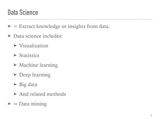
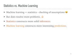
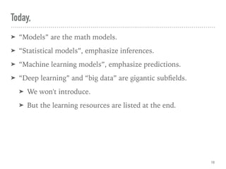


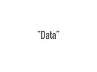
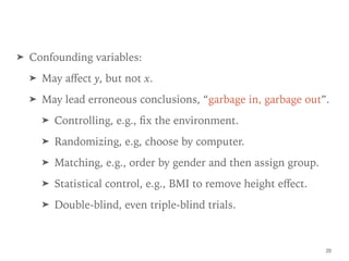


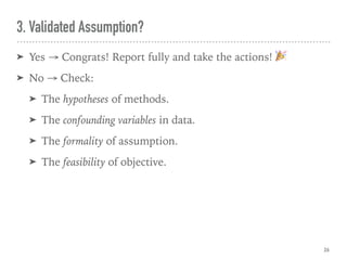


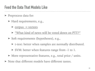

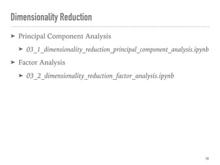
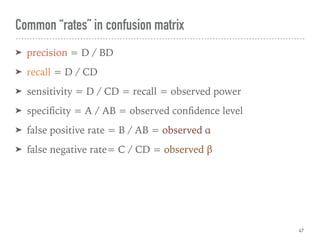
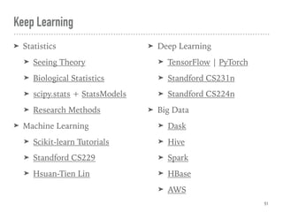
![Confusion matrix, where A = 002 = C[0, 0]
46
predicted -
AC
predicted +
BD
actual -
AB
true -
A
false +
B
actual +
CD
false -
C
true +
D](https://image.slidesharecdn.com/datasciencewithpython-180721135020/85/Data-Science-With-Python-46-320.jpg)
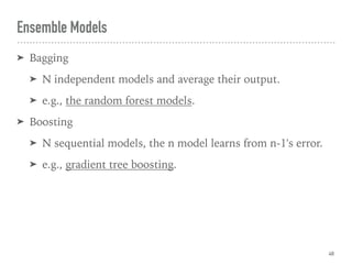
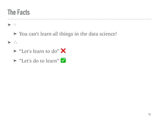


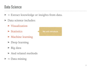
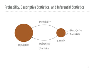
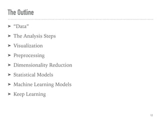
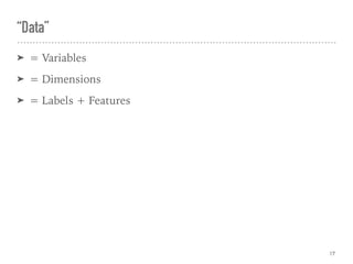
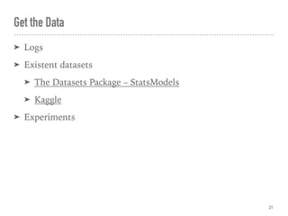
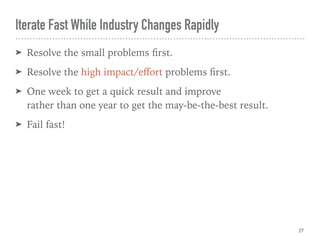
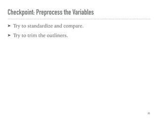
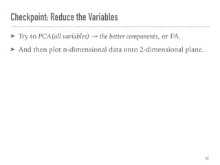
![Confusion matrix, where A = 002 = C[0, 0]
46
predicted -
AC
predicted +
BD
actual -
AB
true -
A
false +
B
actual +
CD
false -
C
true +
D](https://image.slidesharecdn.com/datasciencewithpython-180721135020/75/Data-Science-With-Python-46-2048.jpg)


This document provides an introduction to data science with Python. It discusses key concepts in data science including visualization, statistics, machine learning, deep learning, and big data. Various Python packages are introduced for working with data, including Jupyter, NumPy, SciPy, Matplotlib, Pandas, Scikit-learn and others. The document outlines the main steps in a data science analysis process, including defining assumptions, validating assumptions with data, and iterating. Specific techniques are covered like preprocessing, dimensionality reduction, statistical modeling, and machine learning modeling. The document emphasizes an iterative approach to learning through applying concepts to problems and data.
Introduction to Data Science, its importance in extracting insights and its components like visualization, statistics, machine learning, and big data.
Discussed the relationship between statistics and machine learning, including various statistical concepts and the relevance of machine and deep learning.
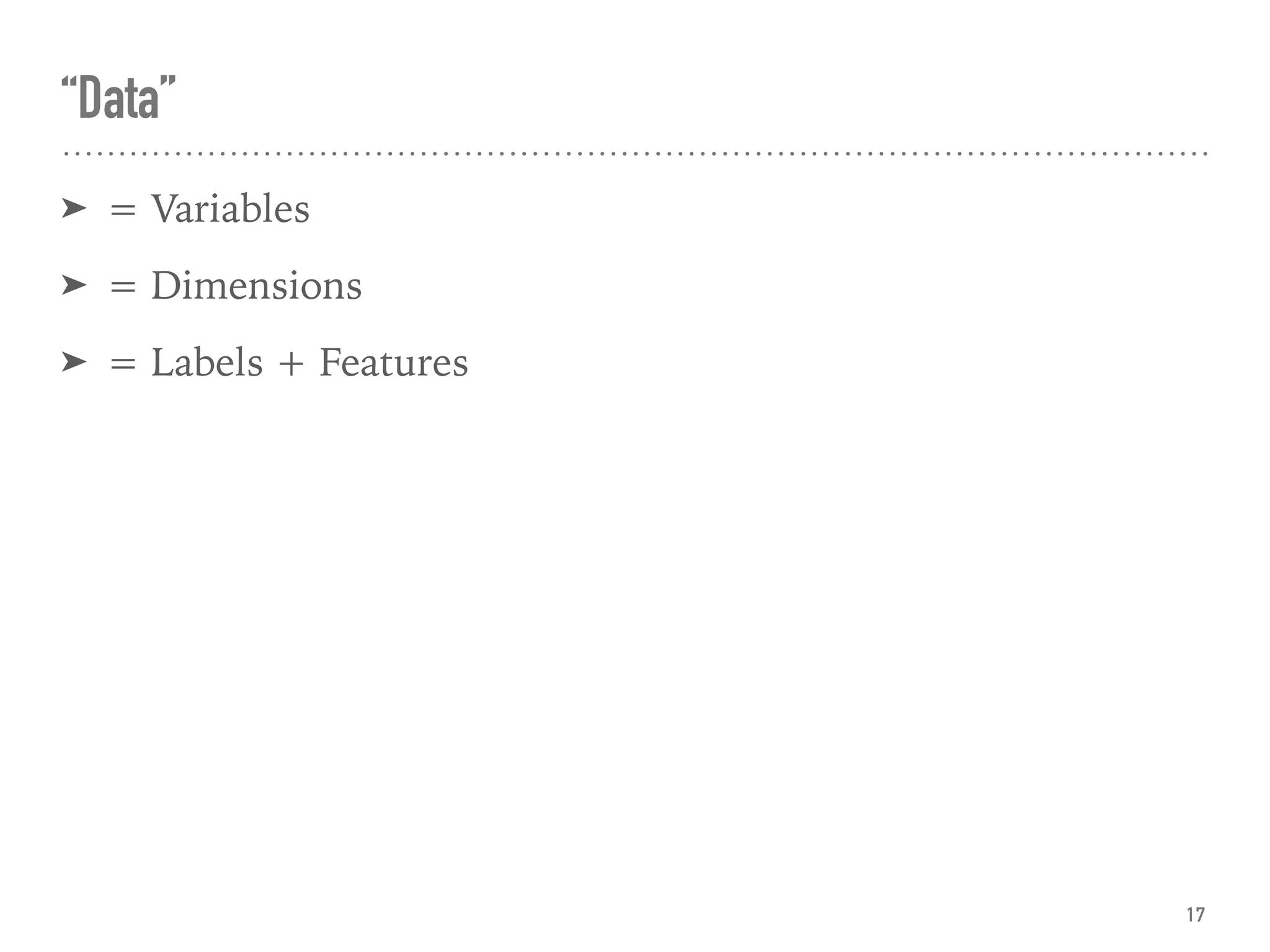
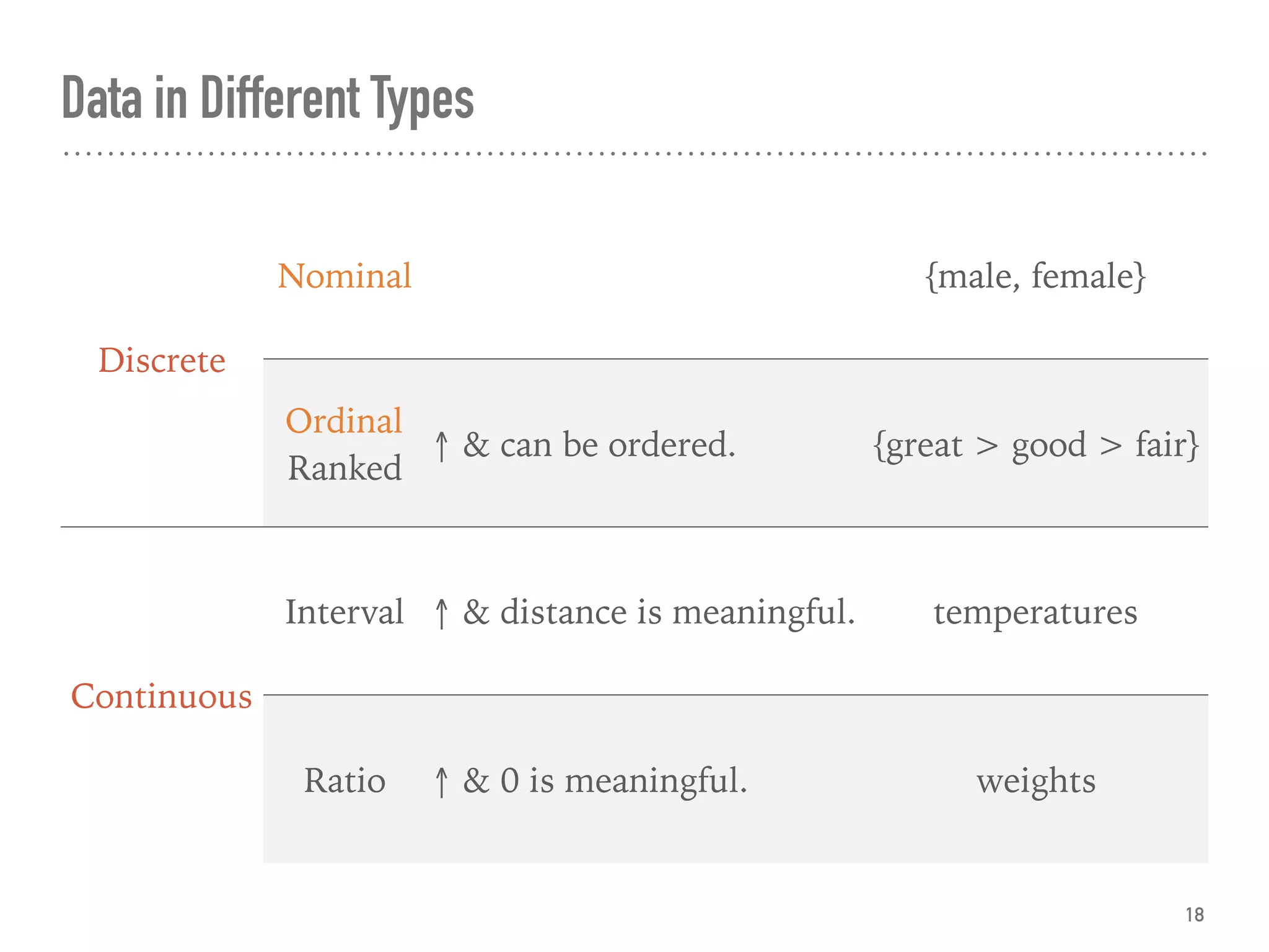
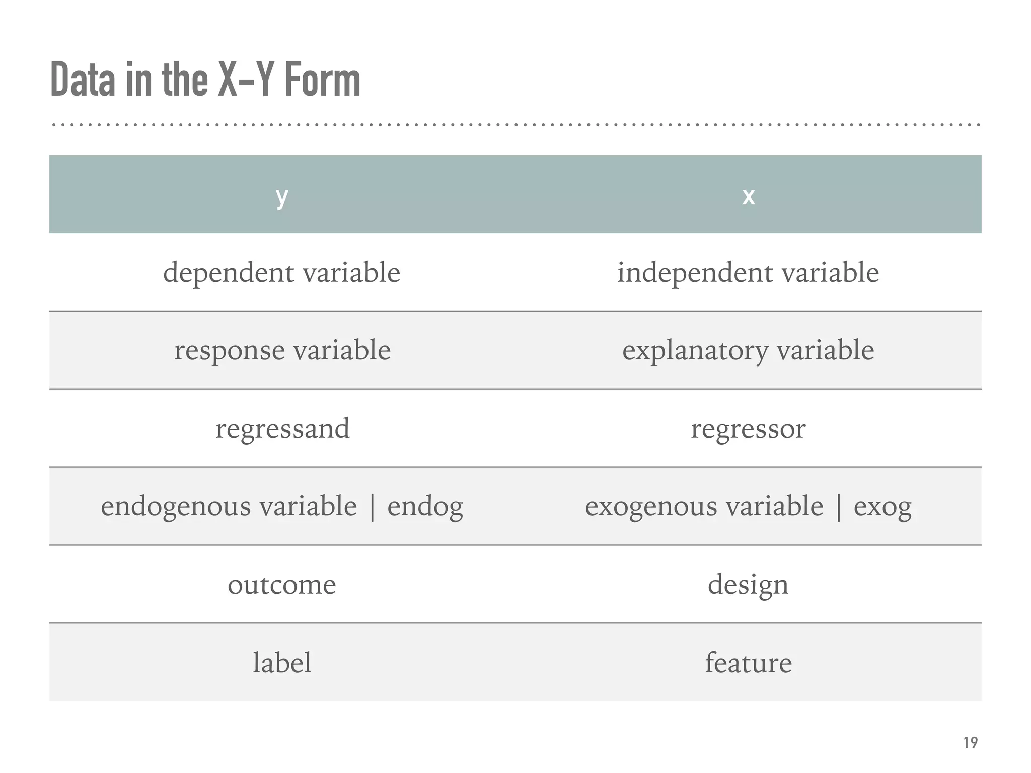
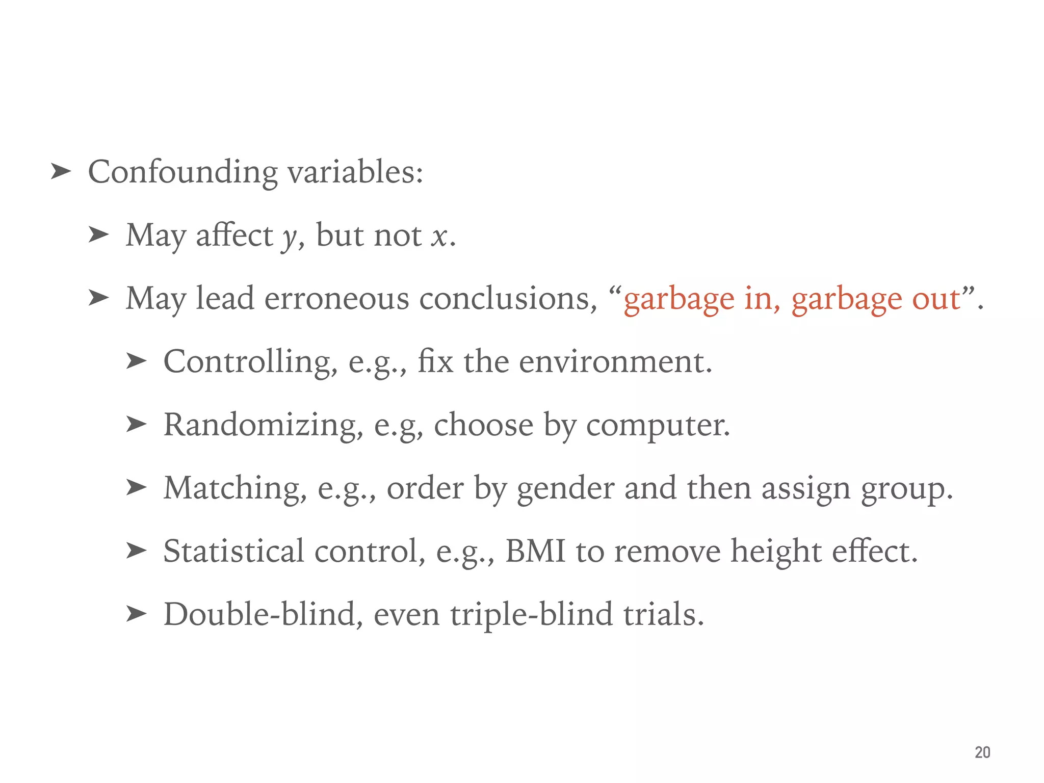
Introduces the concept of data as variables and dimensions, types of data, and confounding variables affecting analysis.
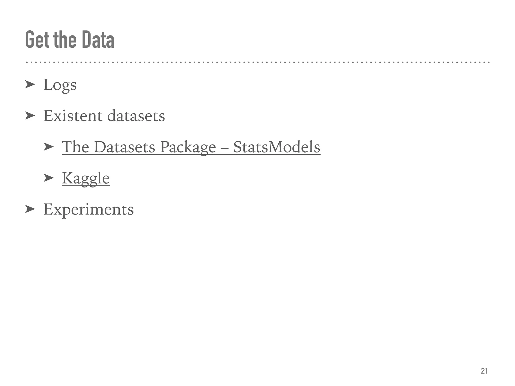
Sources for obtaining data include logs, datasets, Kaggle, and experiments.
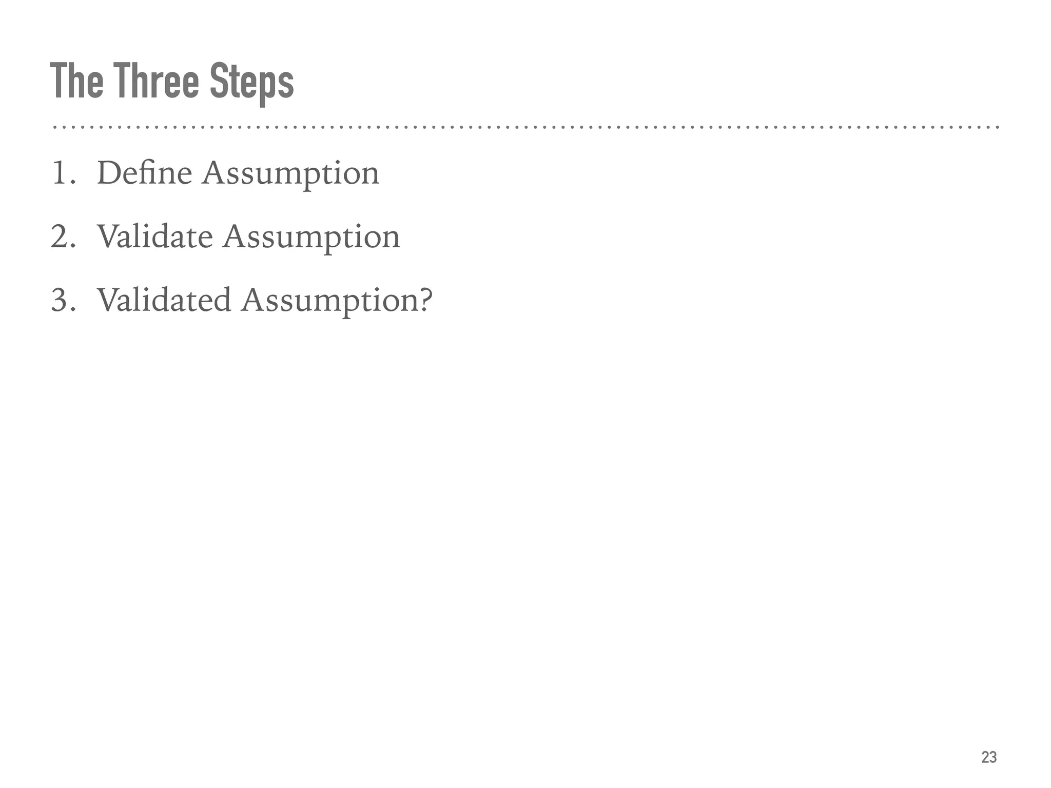
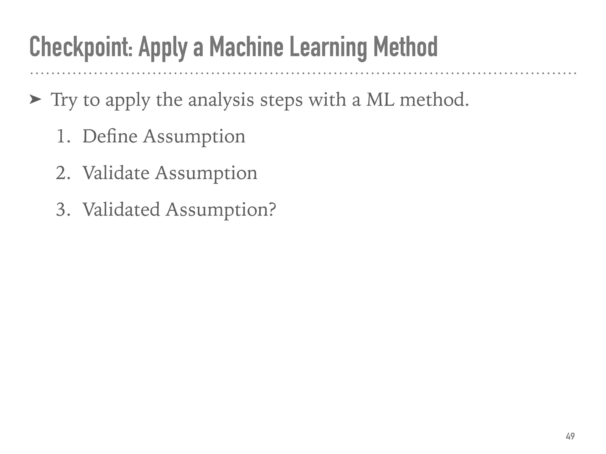
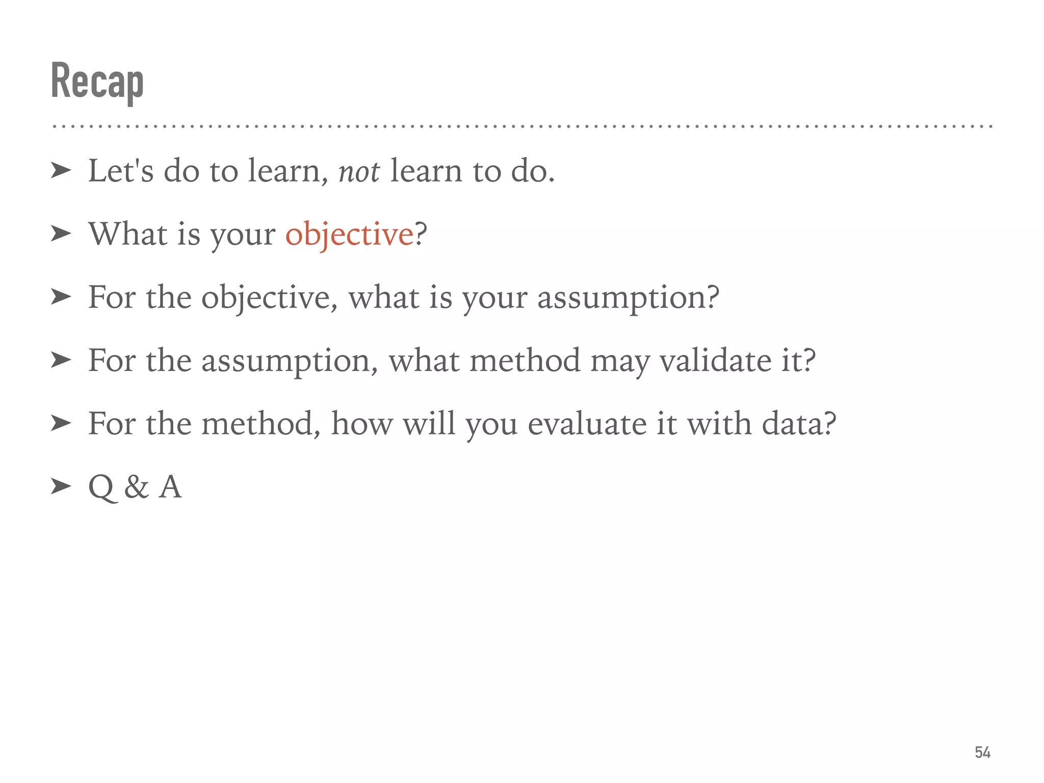
Three essential steps for any analysis: define, validate, and assess assumptions, emphasizing the importance of rapid iterations in responses.
The importance of visualization in data analysis and practical techniques for plotting and making data interpretable.
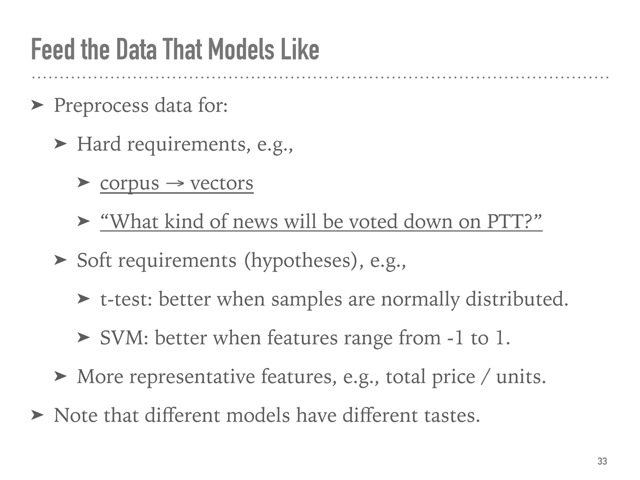
The necessity of preprocessing data to meet model requirements, including standardization and removing outliers to ensure data quality.
Discusses methods to reduce variables for effective analysis, such as PCA and feature extraction.
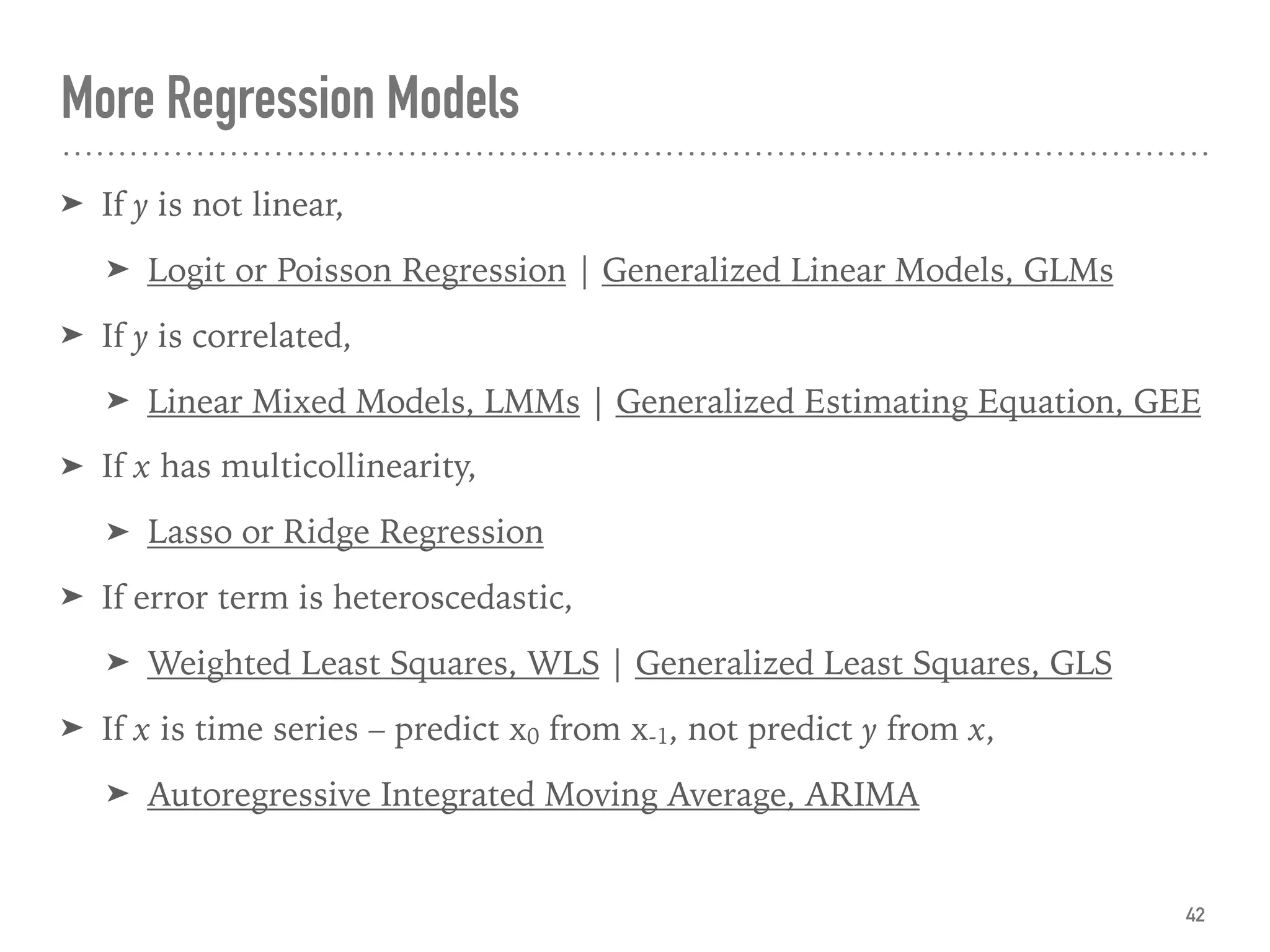
Introduces different statistical modeling approaches including hypothesis testing, regression techniques, and model evaluation methods.
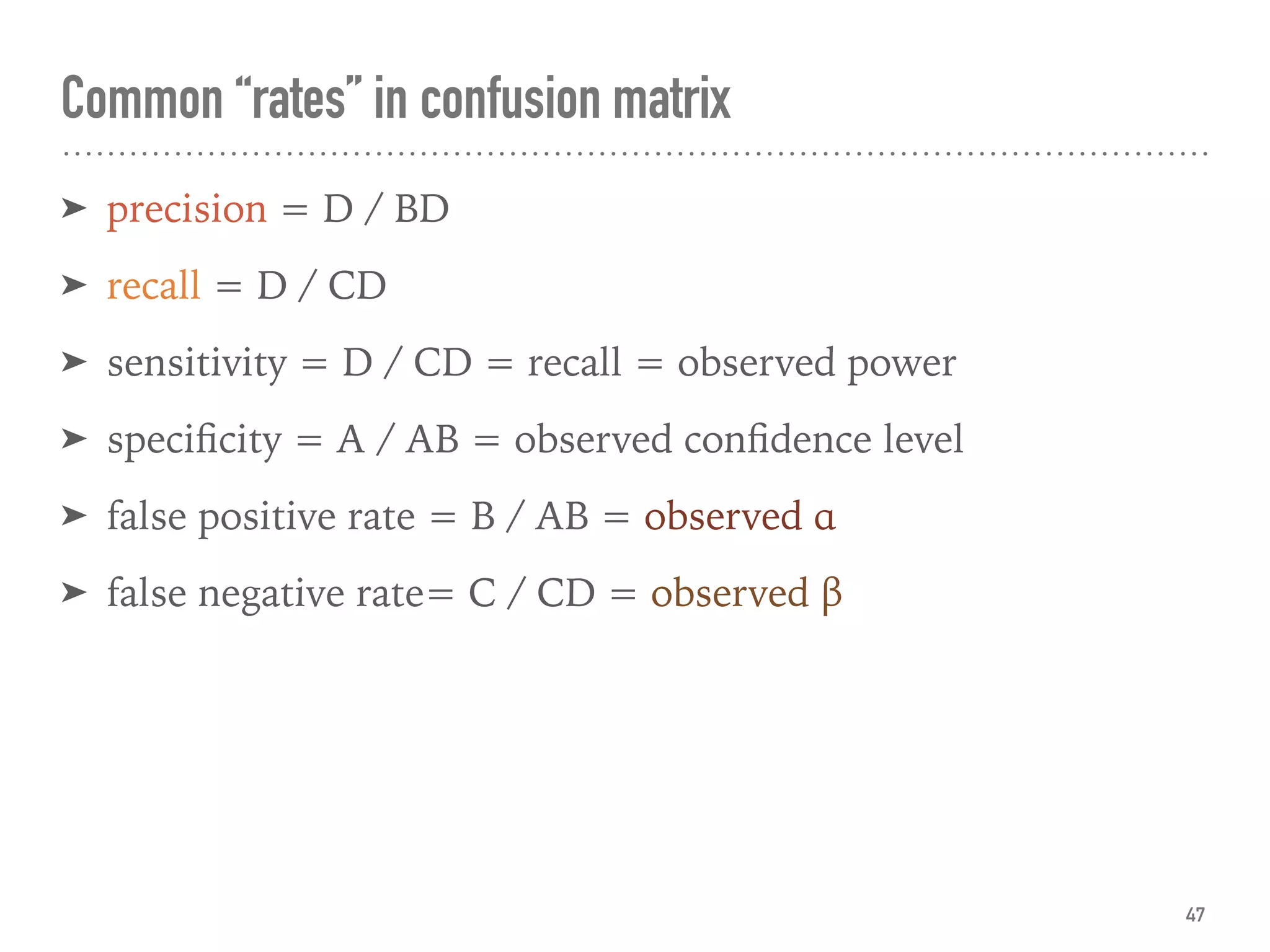
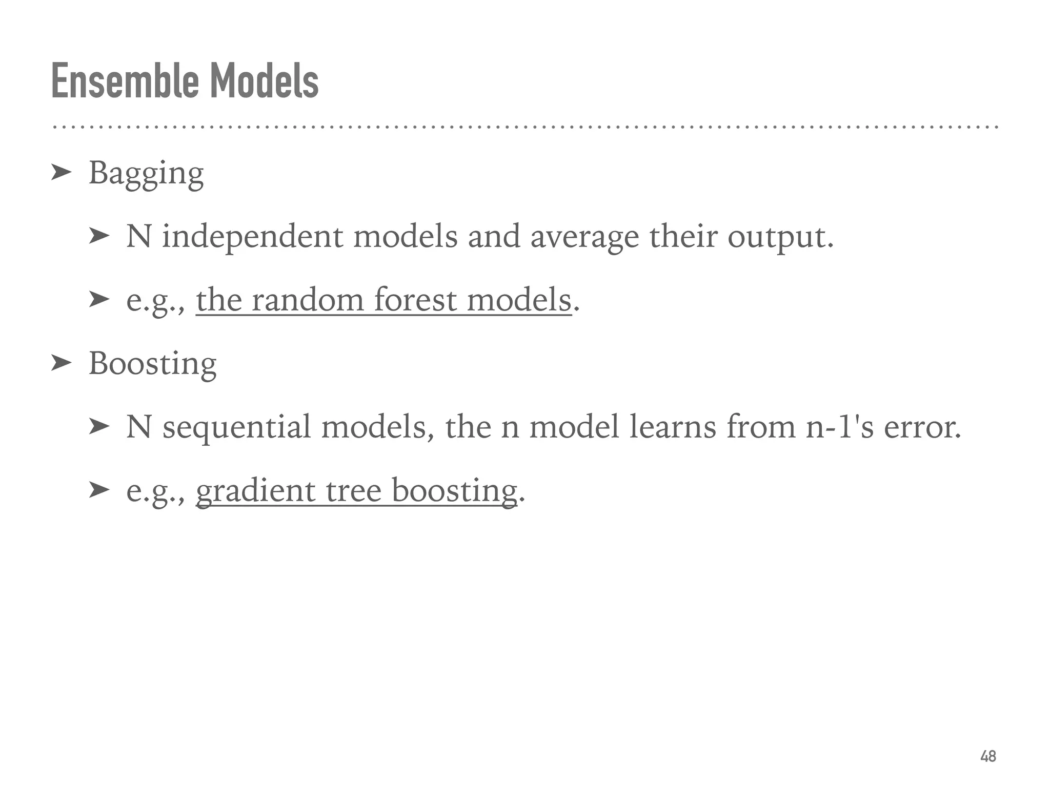
Describes machine learning models for classification, regression, and clustering. Highlights evaluation metrics and methods.
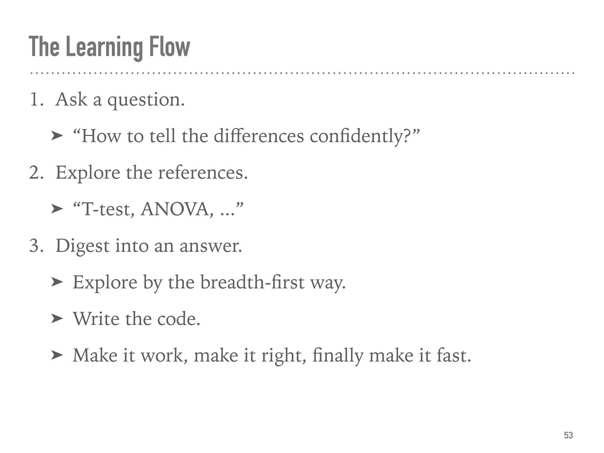
The importance of lifelong learning in statistics, machine learning, and big data, alongside a recap of learning principles.


![RTP_AR_Basic_Learners' Workbook_KS2 [FOR REPRODUCTION] (1).pdf](https://cdn.slidesharecdn.com/ss_thumbnails/rtparbasiclearnersworkbookks2forreproduction1-251016024943-e51a16ac-thumbnail.jpg?width=600ounds&width=560&fit=bounds)


