The document provides an overview of data structures and algorithms in 'C', focusing on searching, sorting, and hashing techniques. It details searching methods like linear and binary search, their algorithms, and various sorting techniques such as selection sort, bubble sort, and merge sort, along with their corresponding algorithms. Additionally, it discusses hashing concepts such as hash tables, hash functions, and collision resolution strategies.
Introduction to data structures, searching types including linear and binary, and a brief on sorting and hashing.
Details on searching methods, describing linear search (time-consuming, O(n)) and binary search (faster, O(log n)) with associated algorithms.
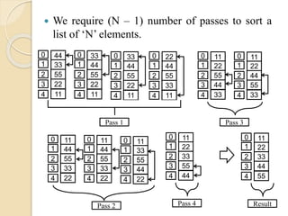
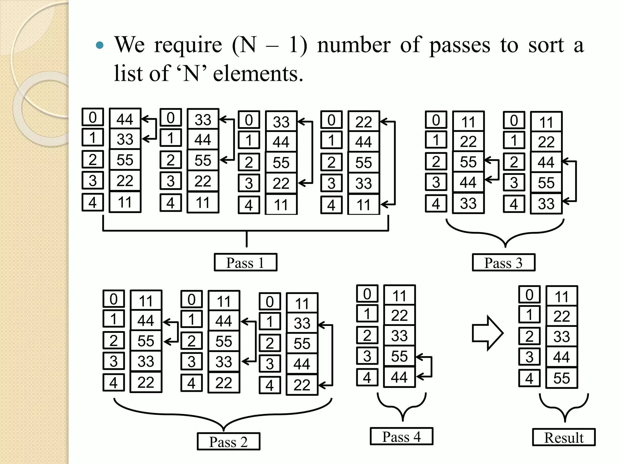
Sorting fundamentals detailing internal vs. external sorting and listing various sorting methods like selection, bubble, and insertion.Description of the selection sort process and algorithm, requiring N-1 passes to sort N elements.
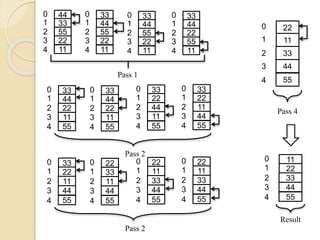
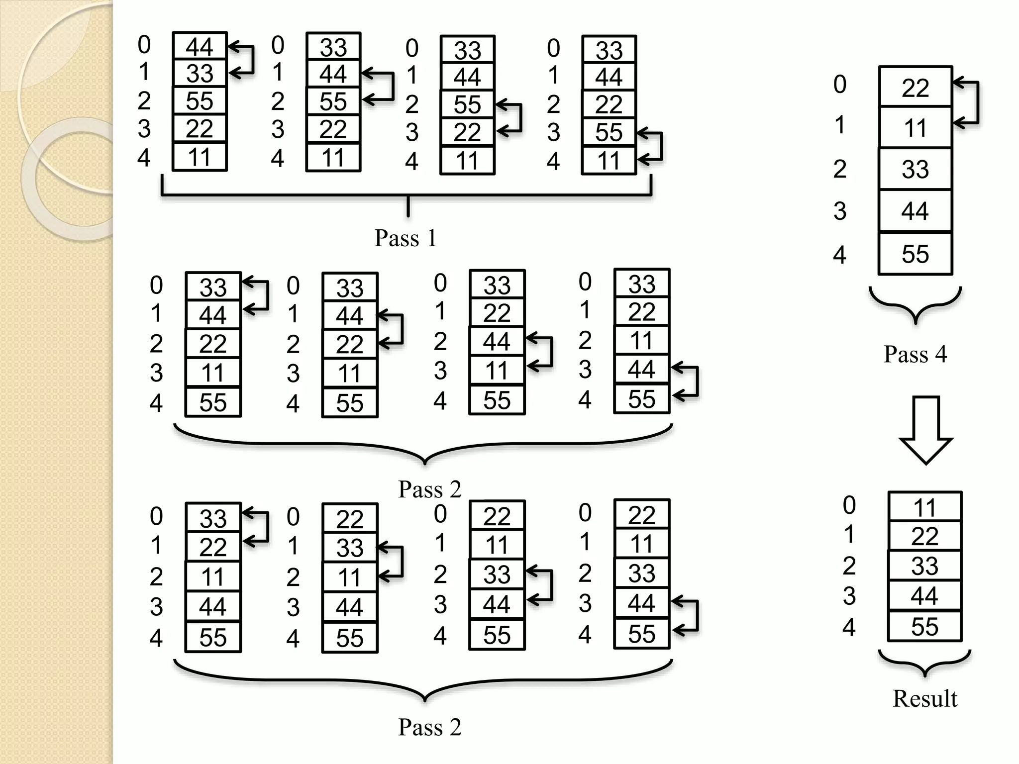
Explanation of bubble sort with its mechanism, including a visual representation of example sorting.
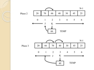
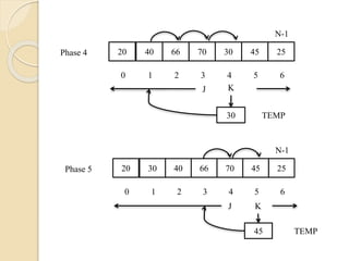
Insertion sort method explained through a card analogy, showcasing sorting phases and the algorithmic steps.
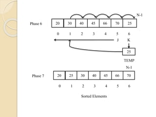
Introduction of radix sort, demonstrating sorting through digit positioning with example data.
Overview of divide and conquer with merge sort, including algorithm detailing and merge process for sorted outputs.
Details on quick sort using pivot selection, illustrating the algorithm with steps for sorting arrays.
Introduction to heap sort, explaining heapify, build_heap and the sorting process through algorithms.
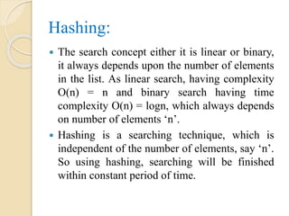
An introduction to hashing as a search technique, discussing its independence from item count.
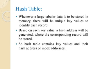
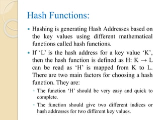
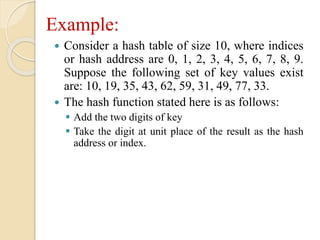
Description of hash tables, hash functions, and collisions, explaining standard methods of hashing.
Various collision resolution methods including closed hashing, linear probing, quadratic probing, and double hashing.
Description of open hashing (chaining), advantages over closed hashing, and how collisions are managed.
Data Structure using
‘C’
Module- III
Prepared by:
Smruti Smaraki Sarangi
Asst. Professor
School of Computer Application
IMS Unison University, Dehradun
2.
Contents
Searching
Typesof search: Linear and Binary
Sorting
Types of Sorting Techniques
Hashing
Hash table and Hash Functions
Types of Hash Functions methods
Collision Resolution Techniques
Different Types of Collision Resolution
Techniques
3.
Searching:
Searching isnothing but find the position of an
element in the given list of elements. Searching
techniques are of two types. That is:
Linear Search
Binary Search
4.
Linear Search:
Whenan element is searched in sequence i.e.
from the beginning of the list to till the end of
the list, it is referred as linear search.
It is a time consuming search, especially when
searched element is present at the end of the list.
The search is successful, when element is found
at some position or unsuccessful, if the element
is not found in the list, based on the presence or
absence of elements in given list.
5.
Algorithm:
LinearSearch(LA, LB, UB,ITEM)
Step 1: Let K, FLAG
Step 2: Set K = LB, FLAG = 0
Step 3: Repeat while(K <= UB)
Step 3.1: if LA[K] = ITEM, then
Step 3.1.1: Set FLAG = 1
Step 3.1.2: Display “ITEM found at”, K
[End of if]
Step 3.2: Set K = K + 1
[End of while]
Step 4: if FLAG = 0, then
Step 4.1: Display “ITEM is not found”.
[End of if]
Step 5: Exit
Note: Here,
linear
array(LA)
upper bound
(UB)
lower bound
(LB)
6.
Binary Search:
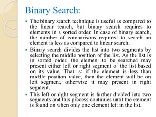
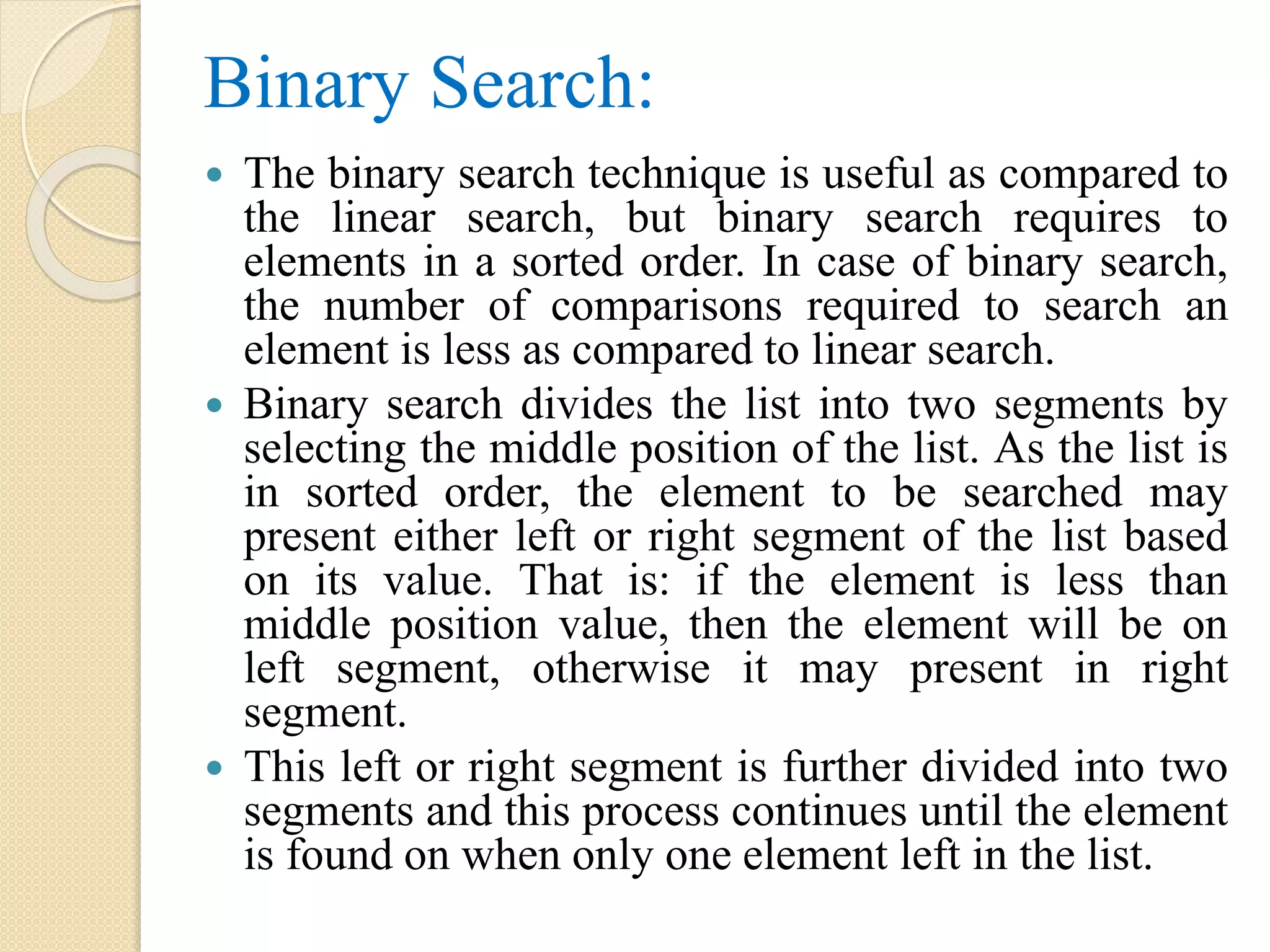
Thebinary search technique is useful as compared to
the linear search, but binary search requires to
elements in a sorted order. In case of binary search,
the number of comparisons required to search an
element is less as compared to linear search.
Binary search divides the list into two segments by
selecting the middle position of the list. As the list is
in sorted order, the element to be searched may
present either left or right segment of the list based
on its value. That is: if the element is less than
middle position value, then the element will be on
left segment, otherwise it may present in right
segment.
This left or right segment is further divided into two
segments and this process continues until the element
is found on when only one element left in the list.
7.
Algorithm:
BinarySearch(LA, LB, UB,ITEM)
Step 1: Let BEG, END, MID, LOC
Step 2: Set BEG = LB, END = UB,
MID = (BEG + END)/2
Step 3: Repeat,
while BEG <= END AND LA[MID] != ITEM
Step 3.1: if ITEM < LA[MID], then set END = MID - 1
Step 3.2: else set BEG = MID + 1
[End of if]
Step 3.3: Set MID = ( BEG + END)/2
[End of while Step 3]
Step 4: if LA[MID] = ITEM, then set LOC = MID
else
set LOC = 0
[End of if]
Step 5: Exit
8.
Sorting:
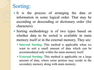
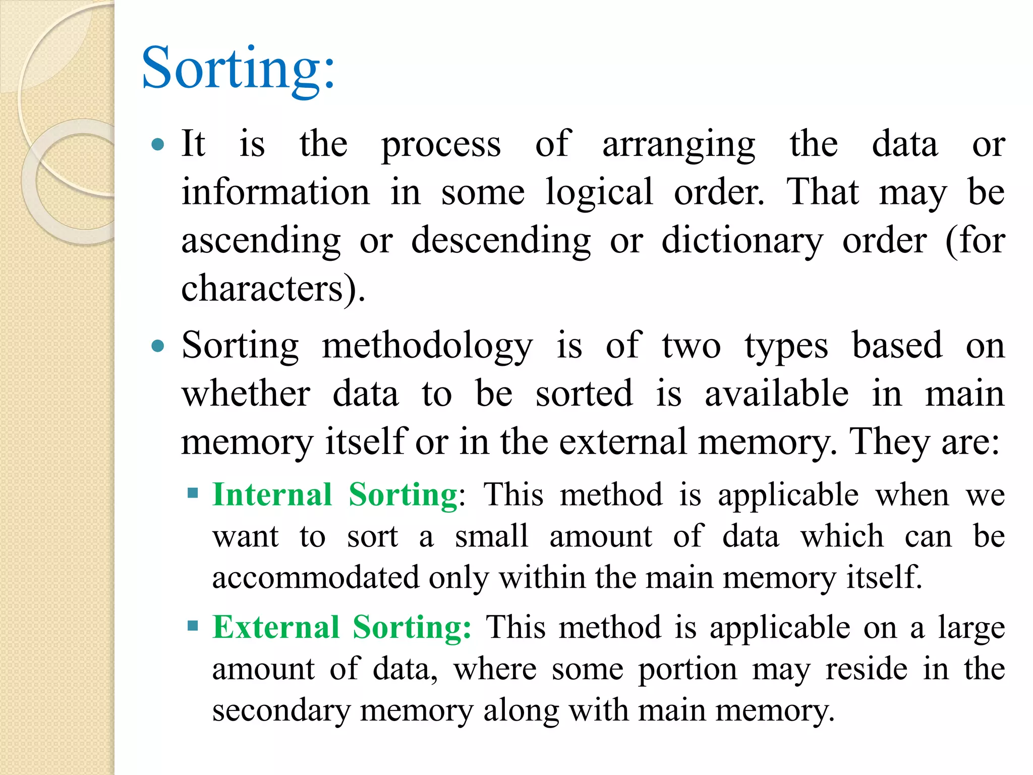
It isthe process of arranging the data or
information in some logical order. That may be
ascending or descending or dictionary order (for
characters).
Sorting methodology is of two types based on
whether data to be sorted is available in main
memory itself or in the external memory. They are:
Internal Sorting: This method is applicable when we
want to sort a small amount of data which can be
accommodated only within the main memory itself.
External Sorting: This method is applicable on a large
amount of data, where some portion may reside in the
secondary memory along with main memory.
Selection Sort:
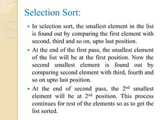
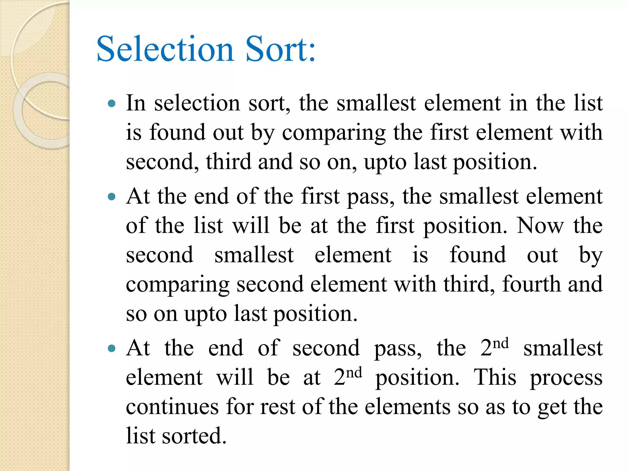
Inselection sort, the smallest element in the list
is found out by comparing the first element with
second, third and so on, upto last position.
At the end of the first pass, the smallest element
of the list will be at the first position. Now the
second smallest element is found out by
comparing second element with third, fourth and
so on upto last position.
At the end of second pass, the 2nd smallest
element will be at 2nd position. This process
continues for rest of the elements so as to get the
list sorted.
Algorithm:
Selection_Sort(A[N])
Step 1:Let I, J, TEMP
Step 2: Repeat for I = 0 to N – 1 increasing by 1
Step 2.1: Repeat for J = I + 1 to N increasing by 1
Step 2.1.1: if A[I] > A[J], then
TEMP = A[I]
A[I] = A[J]
A[J] = TEMP
[End of if]
[End of for]
[End of for]
Step 3: Exit
13.
Bubble Sort:
Inbubble sort, each element is compared with
its adjacent element. If the first element is larger
than the second one then the position of the
elements is interchanged, otherwise it is not
changed. The next element is compared with its
adjacent element and the same process is
repeated for all the elements in the array.
At the end of the pass -1, the largest element in
the list will occupy the last position, at the end
of pass-2, the second largest element will
occupy the 2nd last position and so on.
Algorithm:
Step 1:Let I, K, TEMP
Step 2: Repeat for K = N-2 to 0 decreasing by 1
Step 2.1: Repeat for I = 0 to K increasing by 1
Step 2.1.1: if A[I] > A[I + 1], then
TEMP = A[I]
A[I] = A[I + 1]
A[I + 1] = TEMP
[End of if]
[End of for]
[End of for]
Step 3: Exit
16.
Insertion Sort:
Itis very similar in the way of arranging the
card by a card player.
The card player picks up the cards and inserts
them in the proper position, such that the cards
on hand are sorted.
So, in insertion sort, each element is scanned
and it is inserted in the proper position of
previously sorted sub-array, such that it is in
sorted manner.
17.
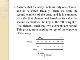
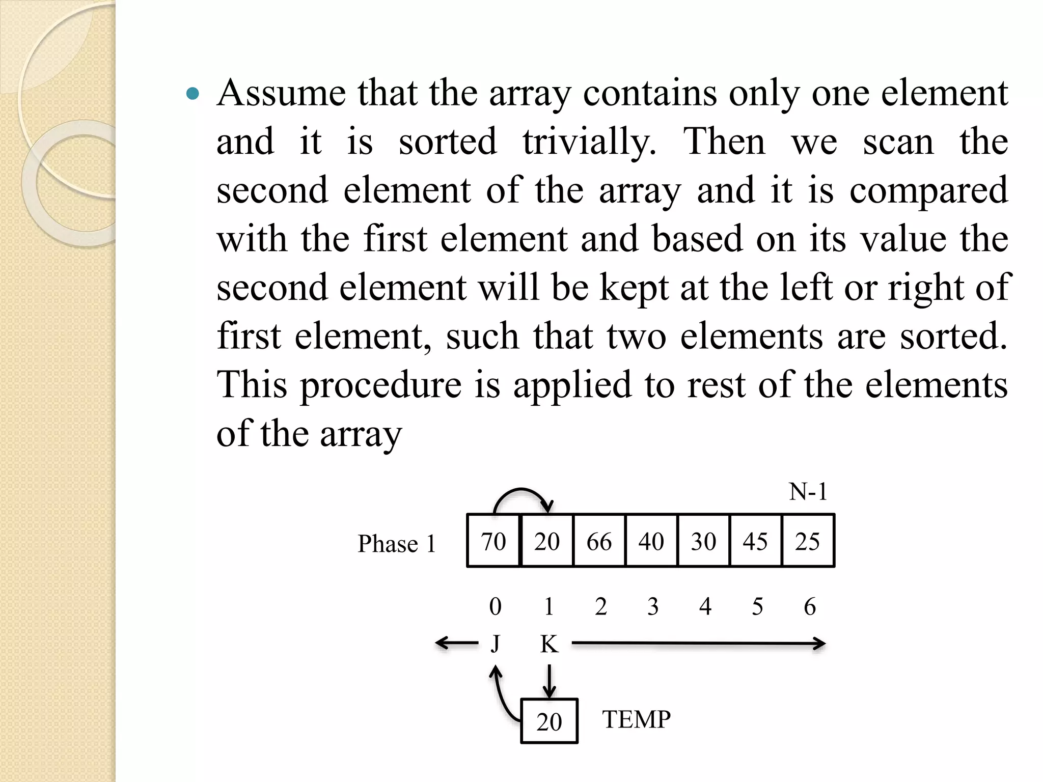
Assume thatthe array contains only one element
and it is sorted trivially. Then we scan the
second element of the array and it is compared
with the first element and based on its value the
second element will be kept at the left or right of
first element, such that two elements are sorted.
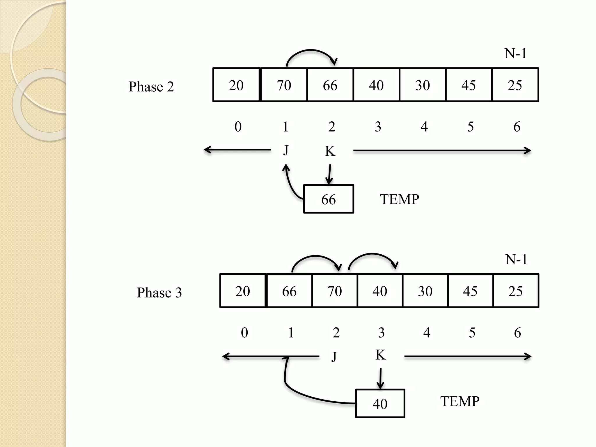
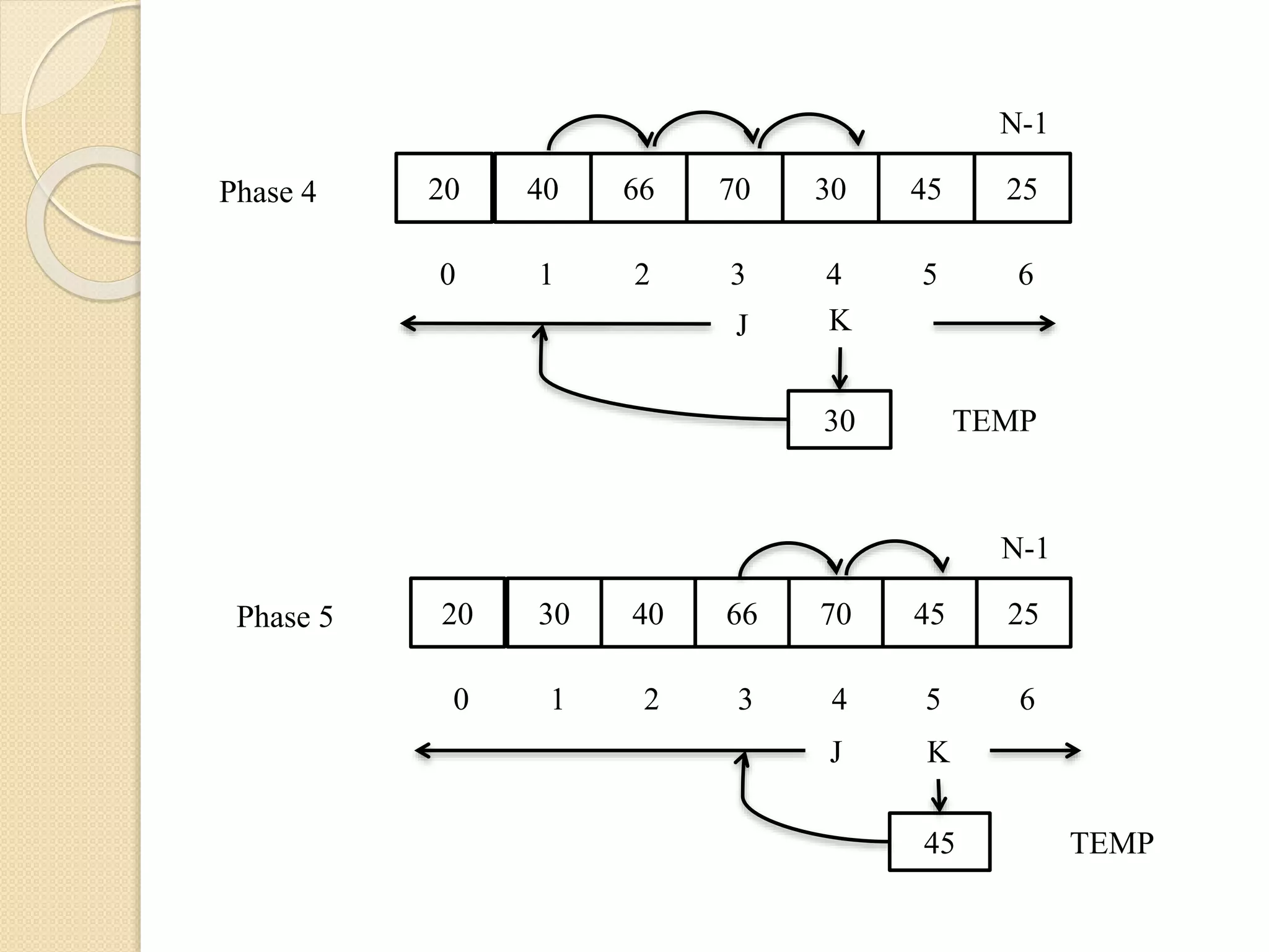
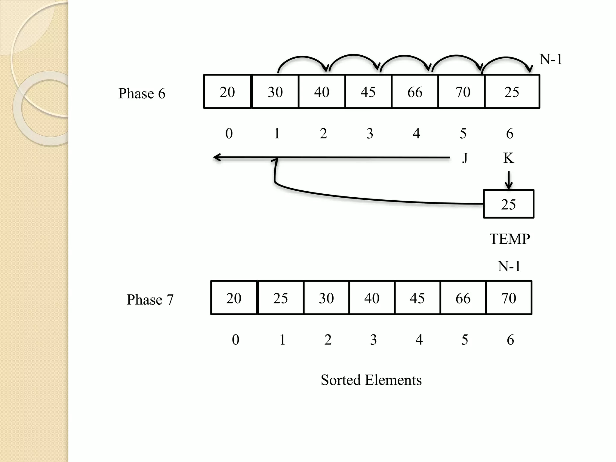
This procedure is applied to rest of the elements
of the array
70 20 66 3040 45 25
N-1
0 1 2 43 5 6
KJ
20 TEMP
Phase 1
Algorithm:
Insertion_Sort(A[N])
Step 1:Let J, K, TEMP
Step 2: Set K = 1
Step 3: Repeat for K = 1 to N – 1 increasing by 1
Set TEMP = A[K]
J = K - 1
Step 3.1: Repeat while ((J >= 0) AND (TEMP < A[J]))
A[J + 1] = A[J]
J = J - 1
[End of while]
Step 3.2: A[J + 1] = TEMP
[End of for]
Step 4: Exit
22.
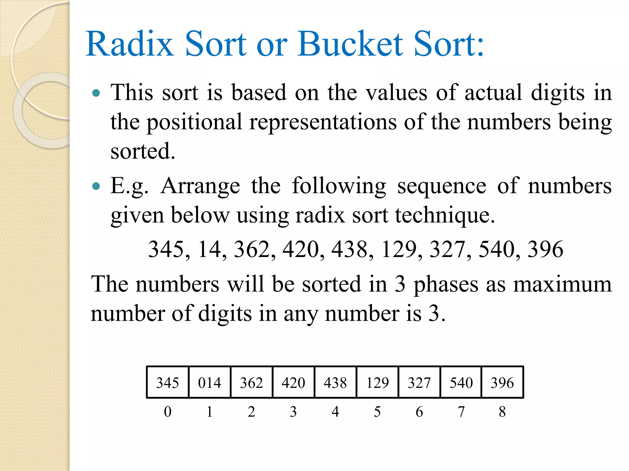
Radix Sort orBucket Sort:
This sort is based on the values of actual digits in
the positional representations of the numbers being
sorted.
E.g. Arrange the following sequence of numbers
given below using radix sort technique.
345, 14, 362, 420, 438, 129, 327, 540, 396
The numbers will be sorted in 3 phases as maximum
number of digits in any number is 3.
345 014 362 420 438 129 327 540 396
0 1 2 3 4 5 6 7 8
23.
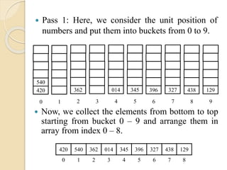
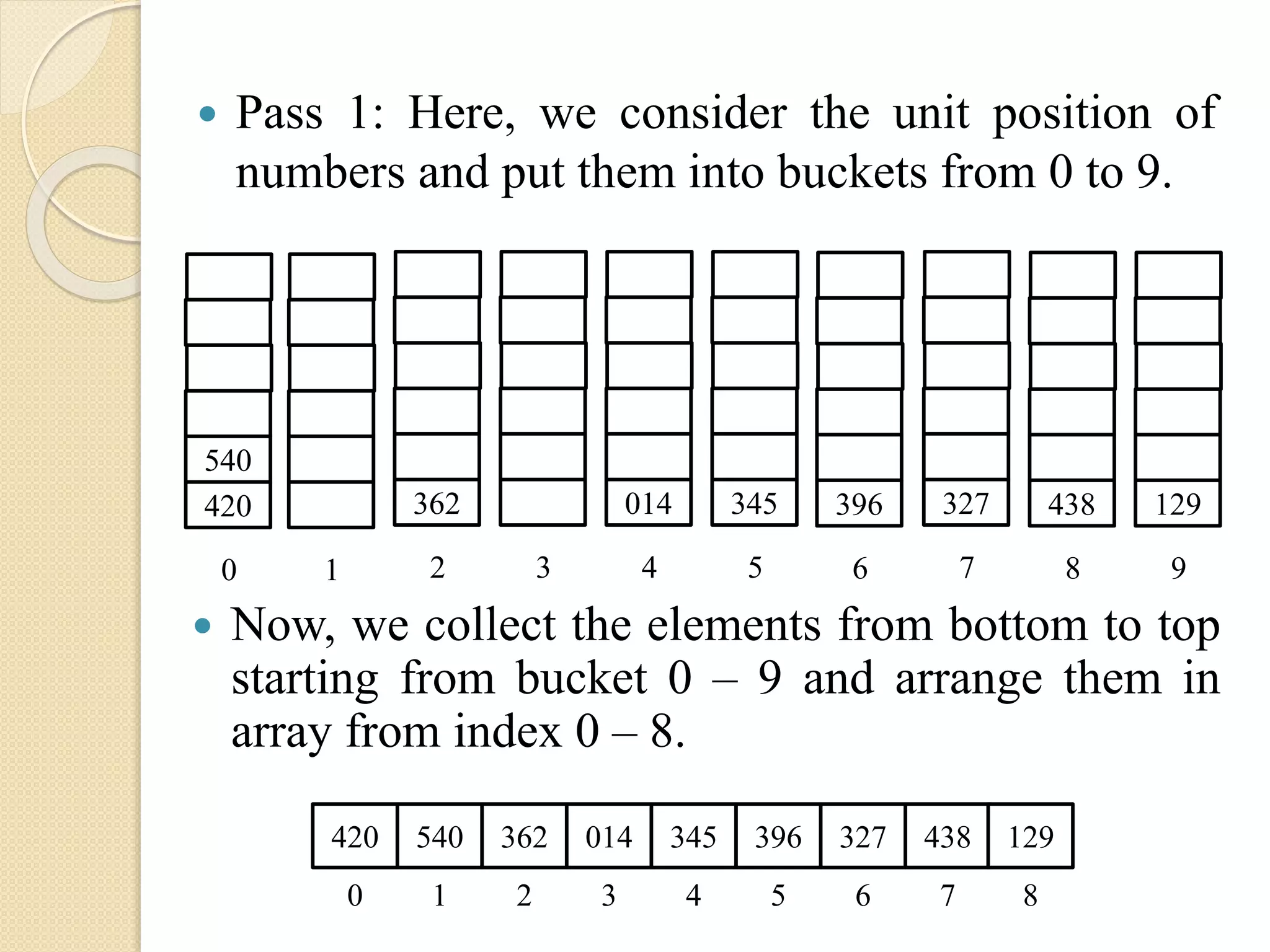
Pass 1:Here, we consider the unit position of
numbers and put them into buckets from 0 to 9.
1 3
396
6
438
8
327
7
014
4
345
5
362
2
540
420
0
129
9
Now, we collect the elements from bottom to top
starting from bucket 0 – 9 and arrange them in
array from index 0 – 8.
420 540 362 014 345 396 327 438 129
0 1 2 3 4 5 6 7 8
24.
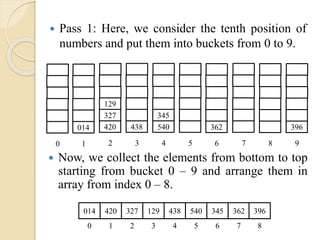
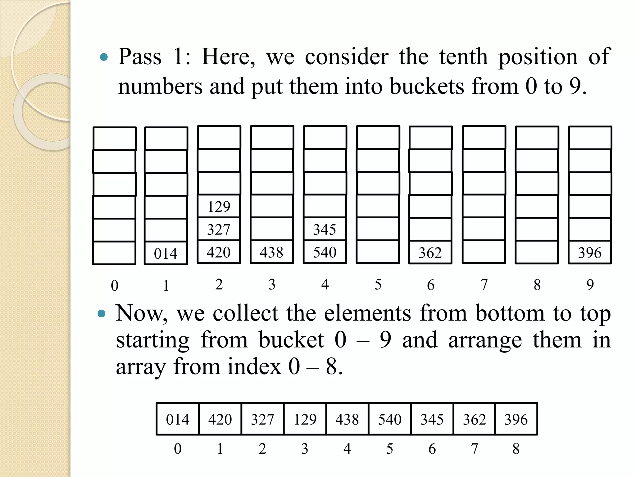
Pass 1:Here, we consider the tenth position of
numbers and put them into buckets from 0 to 9.
014
1
438
3
362
6 87
345
540
4 5
327
129
420
20
396
9
Now, we collect the elements from bottom to top
starting from bucket 0 – 9 and arrange them in
array from index 0 – 8.
014 420 327 129 438 540 345 362 396
0 1 2 3 4 5 6 7 8
25.
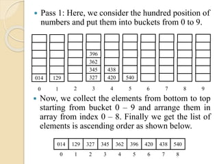
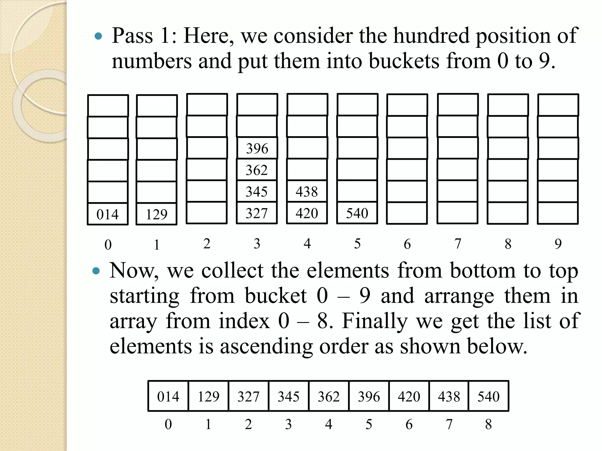
Pass 1:Here, we consider the hundred position of
numbers and put them into buckets from 0 to 9.
129
1
345
362
396
327
3 6 87
438
420
4
540
52
014
0 9
Now, we collect the elements from bottom to top
starting from bucket 0 – 9 and arrange them in
array from index 0 – 8. Finally we get the list of
elements is ascending order as shown below.
014 129 327 345 362 396 420 438 540
0 1 2 3 4 5 6 7 8
26.
Algorithm:
Step 1:Set Large = largest element of the Array
Step 2: Set Num = total number of digits in Large
Step 3: Repeat for Pass = 1 to Num by 1
Step 3.1: Initialize all buckets (0 to 9)
Step 3.2: Repeat for I = 0 to N – 1 by 1
Step 3.2.1: Set Digit = obtain digit at Pass – 1 position
of A[I]
Step 3.2.2: Put A[I] into the bucket Digit
[End of for – Step 3.2]
Step 3.3: Recollect numbers from buckets from 0 to 9
into array A
[End of for – Step 3]
Step 4: Exit
27.
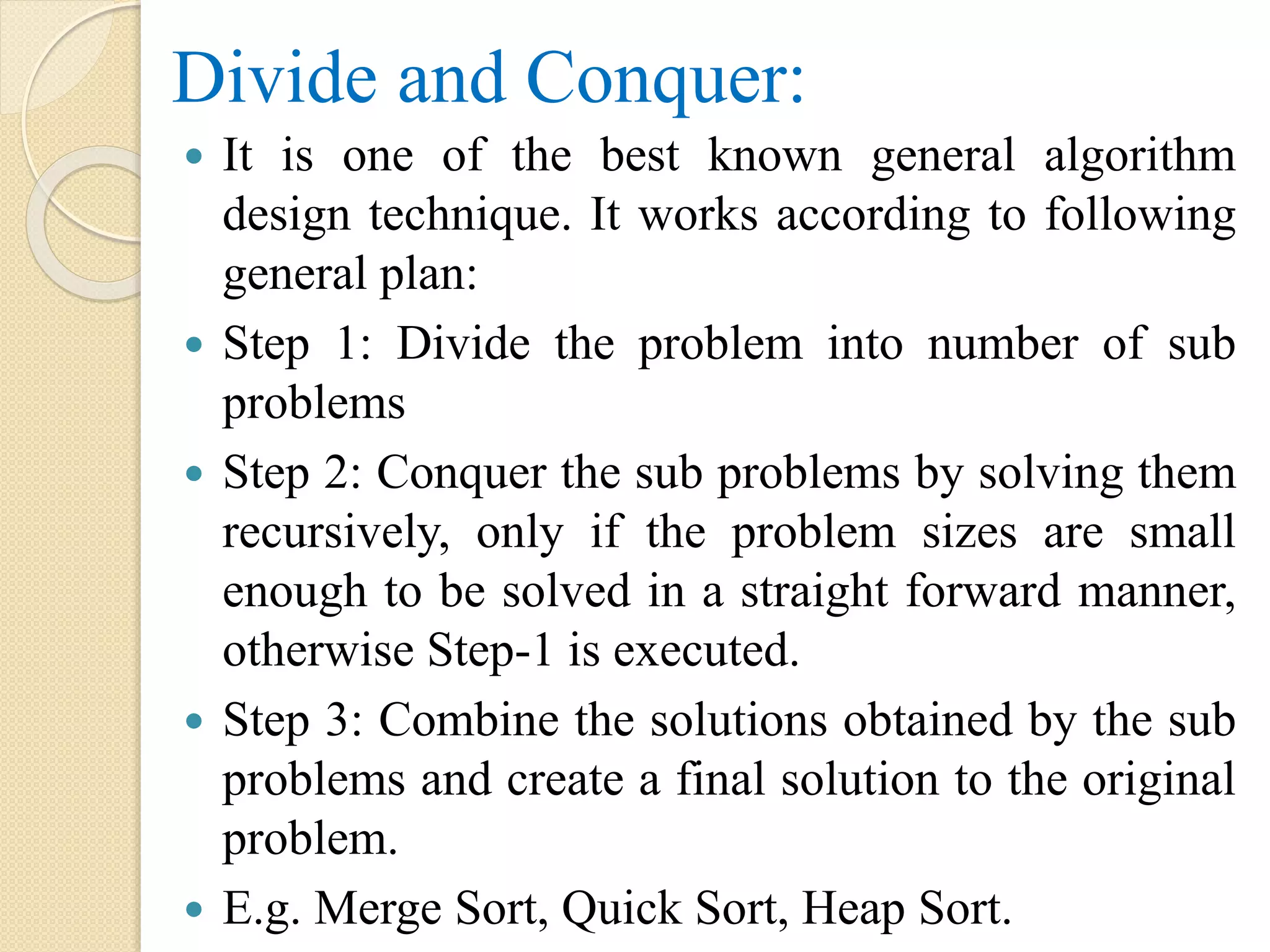
Divide and Conquer:
It is one of the best known general algorithm
design technique. It works according to following
general plan:
Step 1: Divide the problem into number of sub
problems
Step 2: Conquer the sub problems by solving them
recursively, only if the problem sizes are small
enough to be solved in a straight forward manner,
otherwise Step-1 is executed.
Step 3: Combine the solutions obtained by the sub
problems and create a final solution to the original
problem.
E.g. Merge Sort, Quick Sort, Heap Sort.
28.
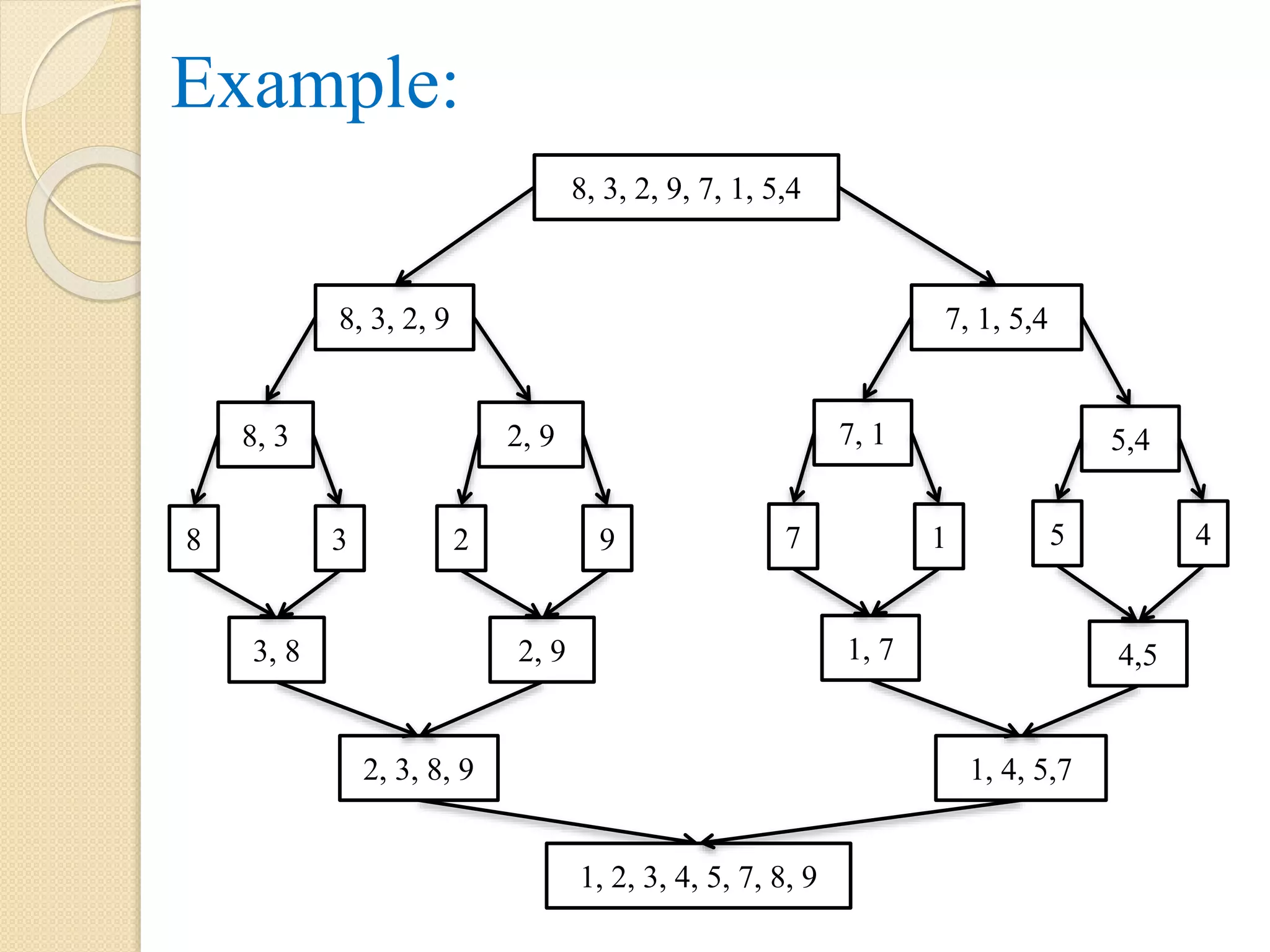
Merge Sort:
Itis a sorting technique, which divides the array
into two sub arrays of sizes 1, 2, 4, …… N by
taking adjacency pairs.
So, we have ‘N’ sub-arrays of size 1, N/2 sub-
arrays of size 2 and so on. This process is
repeated, until there is only one element present.
For accomplishing the whole tasks, we are using
two procedures or algorithms. That is, ‘Merge
Sort’ and ‘Merge’. The procedure ‘Merge’ is used
for combining the sub lists.
29.
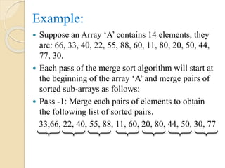
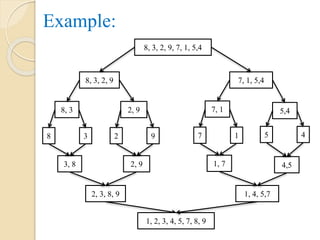
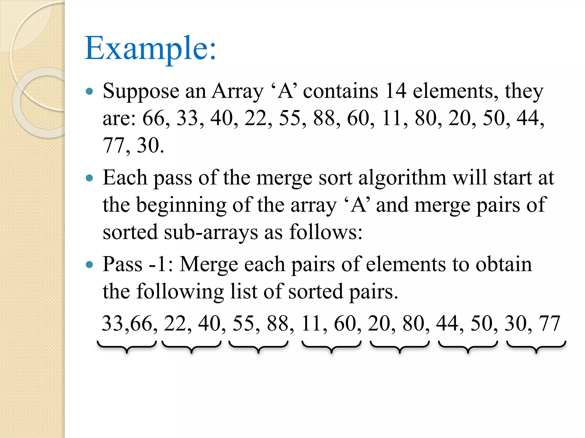
Example:
Suppose anArray ‘A’ contains 14 elements, they
are: 66, 33, 40, 22, 55, 88, 60, 11, 80, 20, 50, 44,
77, 30.
Each pass of the merge sort algorithm will start at
the beginning of the array ‘A’ and merge pairs of
sorted sub-arrays as follows:
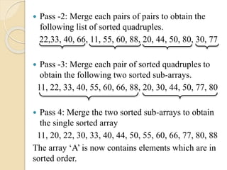
Pass -1: Merge each pairs of elements to obtain
the following list of sorted pairs.
33,66, 22, 40, 55, 88, 11, 60, 20, 80, 44, 50, 30, 77
30.
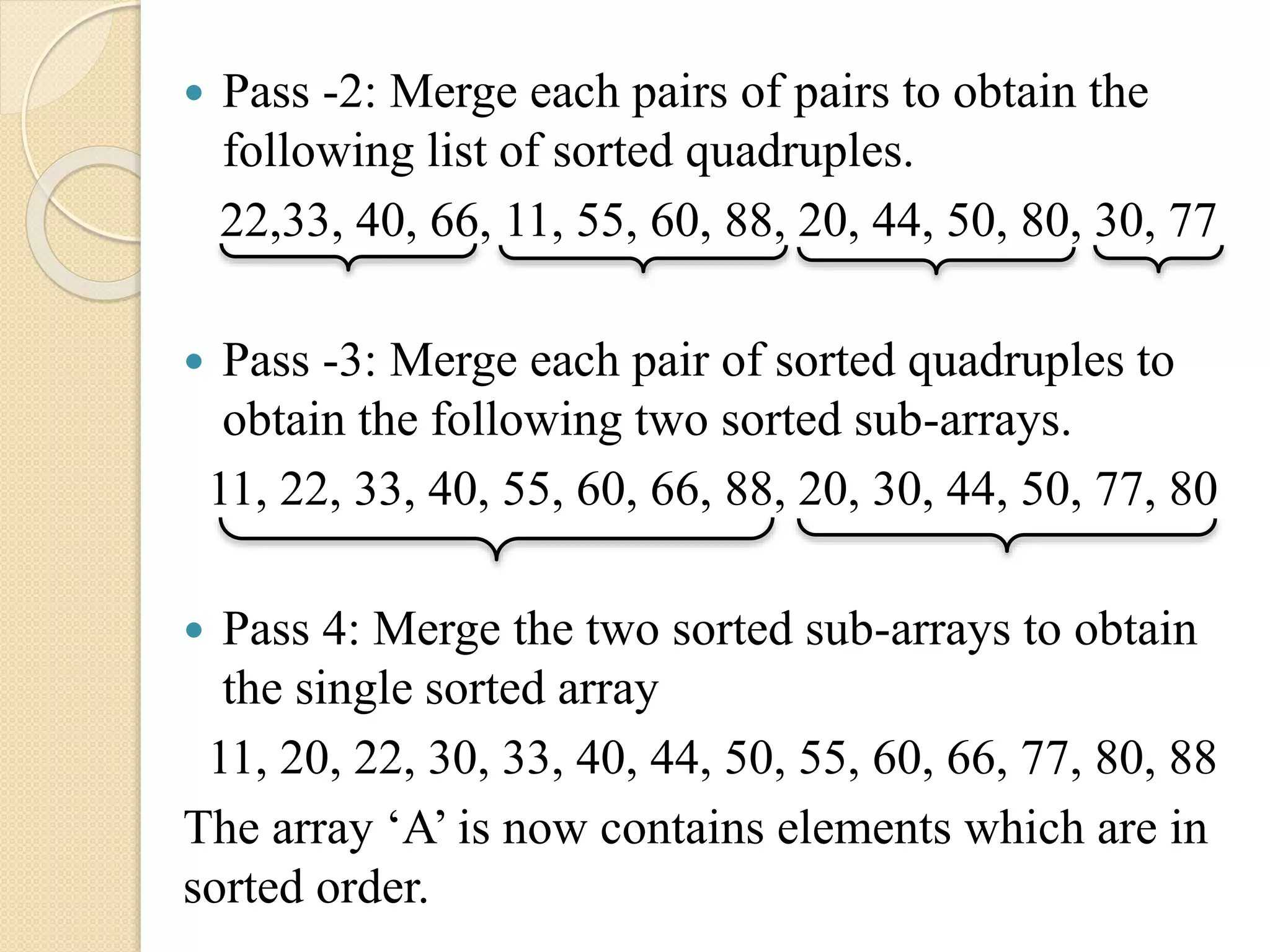
Pass -2:Merge each pairs of pairs to obtain the
following list of sorted quadruples.
22,33, 40, 66, 11, 55, 60, 88, 20, 44, 50, 80, 30, 77
Pass -3: Merge each pair of sorted quadruples to
obtain the following two sorted sub-arrays.
11, 22, 33, 40, 55, 60, 66, 88, 20, 30, 44, 50, 77, 80
Pass 4: Merge the two sorted sub-arrays to obtain
the single sorted array
11, 20, 22, 30, 33, 40, 44, 50, 55, 60, 66, 77, 80, 88
The array ‘A’ is now contains elements which are in
sorted order.
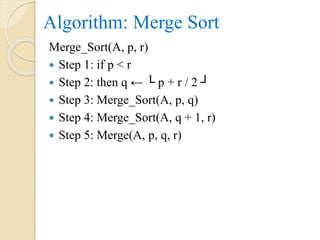
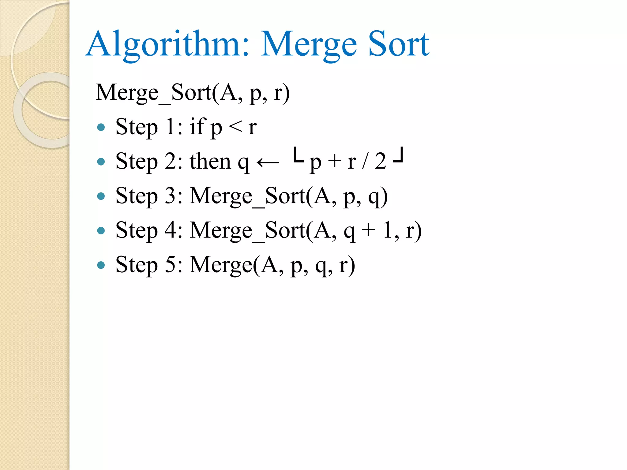
Algorithm: Merge Sort
Merge_Sort(A,p, r)
Step 1: if p < r
Step 2: then q ← └ p + r / 2 ┘
Step 3: Merge_Sort(A, p, q)
Step 4: Merge_Sort(A, q + 1, r)
Step 5: Merge(A, p, q, r)
33.
Algorithm: Merge
Merge (A,p, q, r)
Step 1: n1 ← q – p + 1
Step 2: n2 ← r - q
Step 3: create arrays L[1…n1 + 1] and R[1…n2 + 1]
Step 4: for i ← 1 to n1
Step 5: do L[i] ← A[p + i – 1]
Step 6: for j ← 1 to n2
Step 7: do R[j] ← A[q + j]
Step 8: L[n1 + 1] ← ∞
Step 9: R[n2 + 1] ← ∞
Step 10: i ← 1
34.
Step 11:j ← 1
Step 12: for k ← p to r
Step 13: do if L[i] ≤ R[j]
Step 14: then A[k] ← L[i]
Step 15: i ← i + 1
Step 16: else A[k] ← R[j]
Step 17: j ← j + 1
Time complexity of Merge Sort:
The time complexity of Merge Sort (total time) is:
T(n) = θ(nlogn) and total cost = cnlogn.
Merge procedure on an ‘n’ elements sub-array
takes time θ(n).
35.
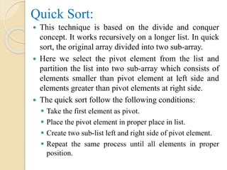
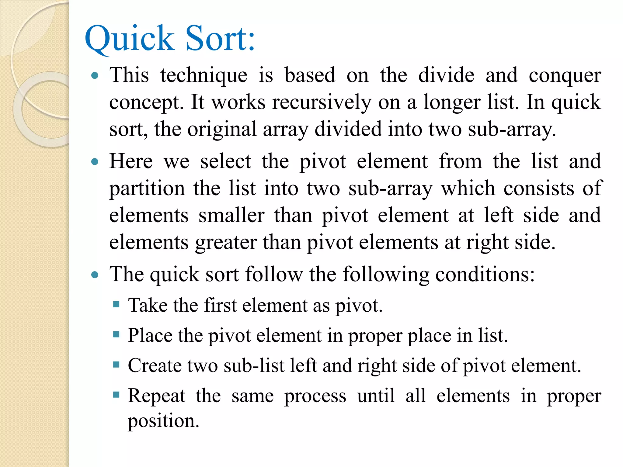
Quick Sort:
Thistechnique is based on the divide and conquer
concept. It works recursively on a longer list. In quick
sort, the original array divided into two sub-array.
Here we select the pivot element from the list and
partition the list into two sub-array which consists of
elements smaller than pivot element at left side and
elements greater than pivot elements at right side.
The quick sort follow the following conditions:
Take the first element as pivot.
Place the pivot element in proper place in list.
Create two sub-list left and right side of pivot element.
Repeat the same process until all elements in proper
position.
36.
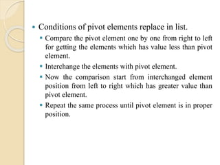
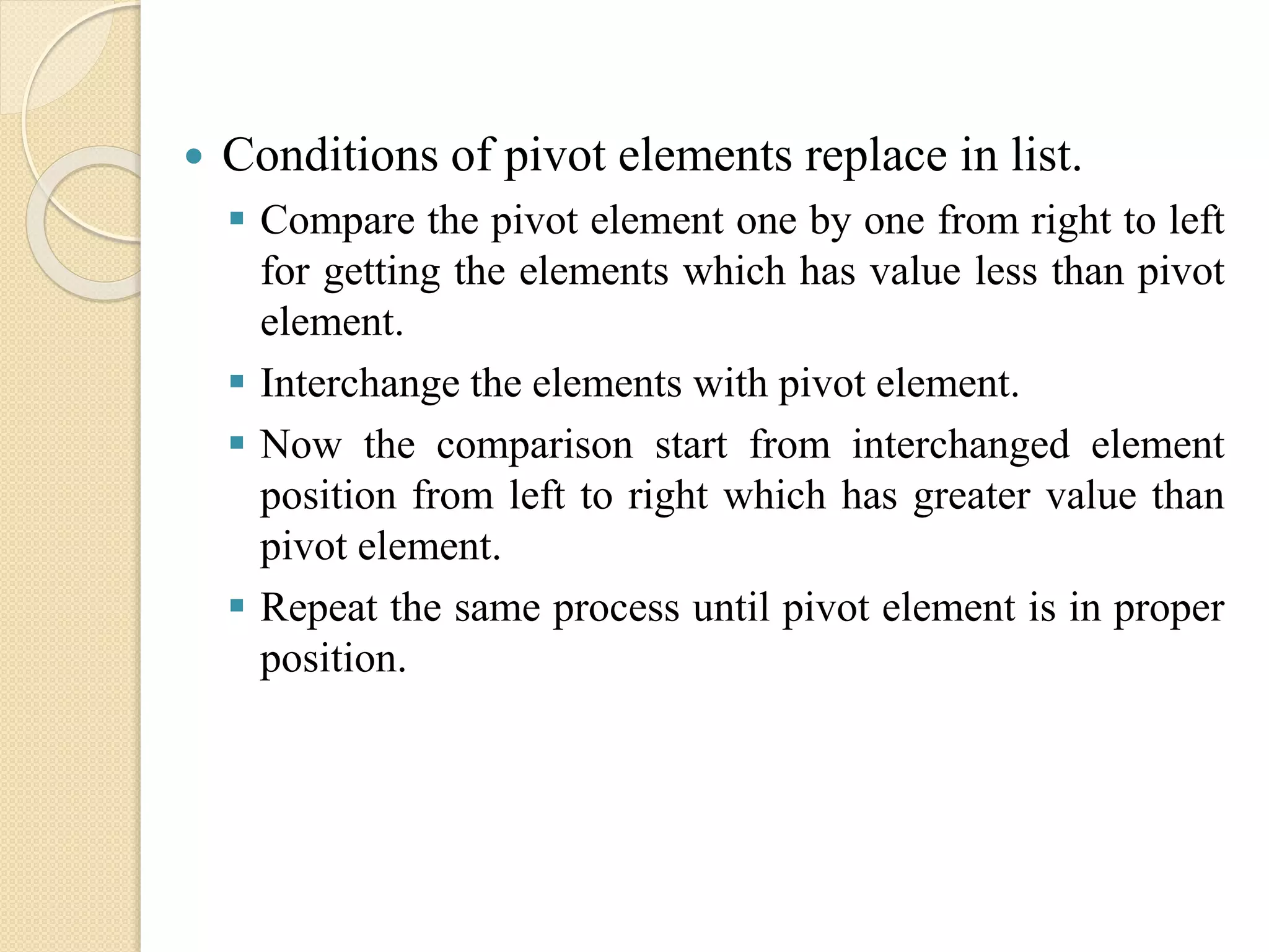
Conditions ofpivot elements replace in list.
Compare the pivot element one by one from right to left
for getting the elements which has value less than pivot
element.
Interchange the elements with pivot element.
Now the comparison start from interchanged element
position from left to right which has greater value than
pivot element.
Repeat the same process until pivot element is in proper
position.
37.
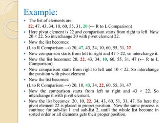
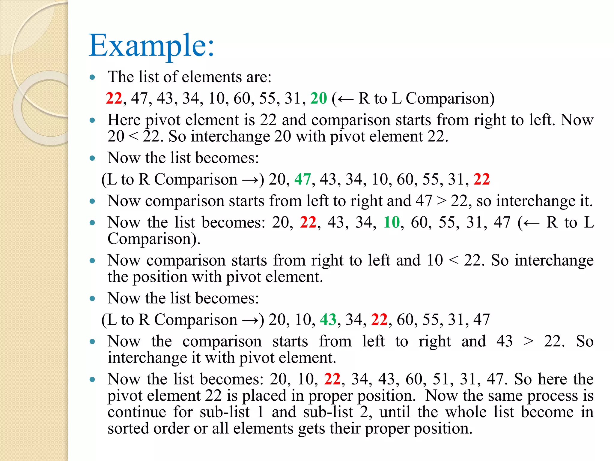
Example:
The listof elements are:
22, 47, 43, 34, 10, 60, 55, 31, 20 (← R to L Comparison)
Here pivot element is 22 and comparison starts from right to left. Now
20 < 22. So interchange 20 with pivot element 22.
Now the list becomes:
(L to R Comparison →) 20, 47, 43, 34, 10, 60, 55, 31, 22
Now comparison starts from left to right and 47 > 22, so interchange it.
Now the list becomes: 20, 22, 43, 34, 10, 60, 55, 31, 47 (← R to L
Comparison).
Now comparison starts from right to left and 10 < 22. So interchange
the position with pivot element.
Now the list becomes:
(L to R Comparison →) 20, 10, 43, 34, 22, 60, 55, 31, 47
Now the comparison starts from left to right and 43 > 22. So
interchange it with pivot element.
Now the list becomes: 20, 10, 22, 34, 43, 60, 51, 31, 47. So here the
pivot element 22 is placed in proper position. Now the same process is
continue for sub-list 1 and sub-list 2, until the whole list become in
sorted order or all elements gets their proper position.
38.
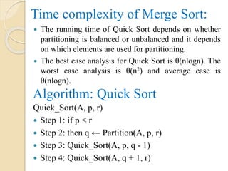
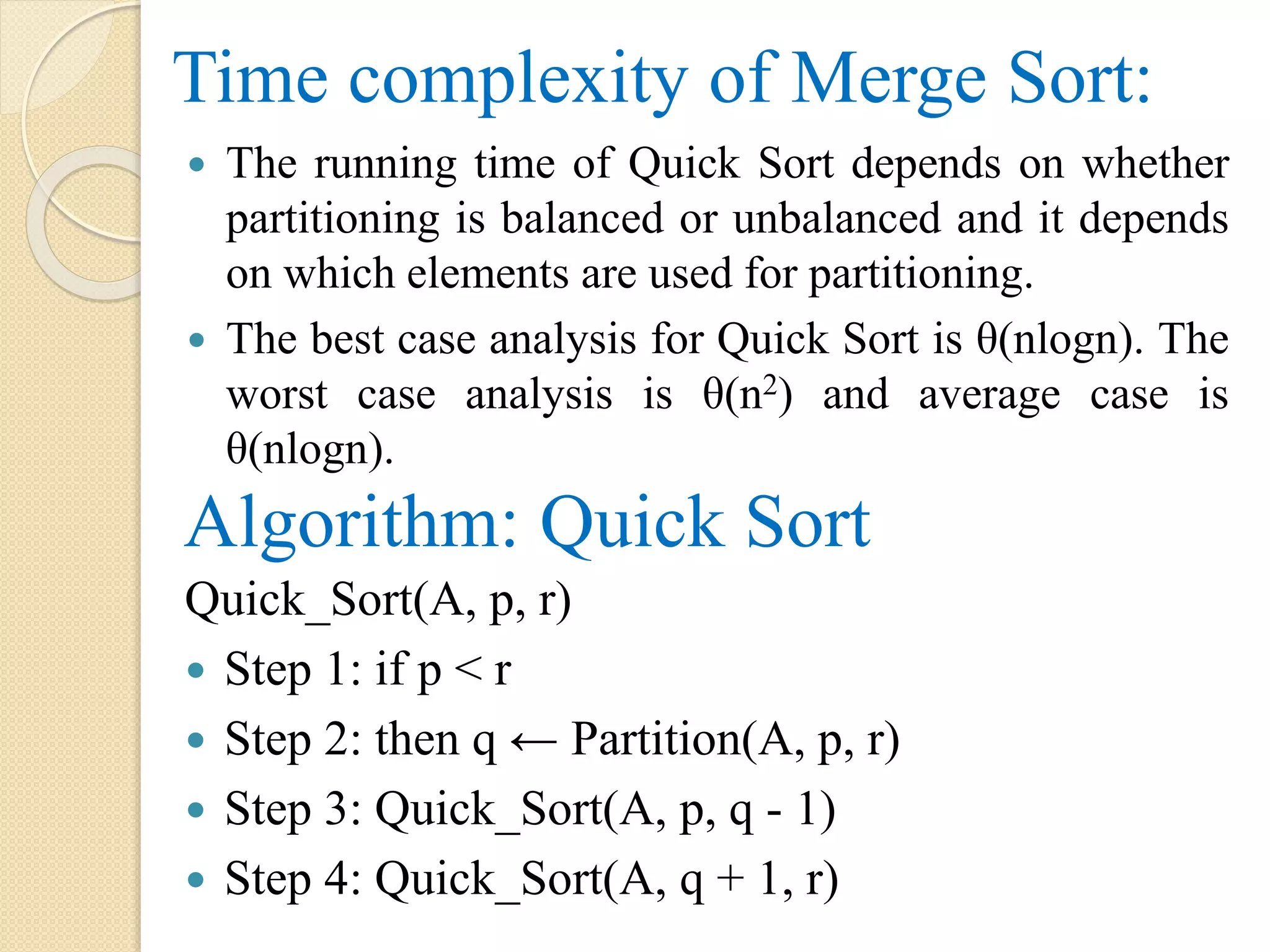
Time complexity ofMerge Sort:
The running time of Quick Sort depends on whether
partitioning is balanced or unbalanced and it depends
on which elements are used for partitioning.
The best case analysis for Quick Sort is θ(nlogn). The
worst case analysis is θ(n2) and average case is
θ(nlogn).
Algorithm: Quick Sort
Quick_Sort(A, p, r)
Step 1: if p < r
Step 2: then q ← Partition(A, p, r)
Step 3: Quick_Sort(A, p, q - 1)
Step 4: Quick_Sort(A, q + 1, r)
39.
Algorithm: Partition
Partition(A, p,r)
Step 1: x ← A[r]
Step 2: i ← p - 1
Step 3: j ← p to r - 1
Step 4: do if A[j] ≤ x
Step 5: then i ← i + 1
Step 6: exchange A[i] ↔ A[j]
Step 7: exchange A[i + 1] ↔ A[r]
Step 8: return
40.
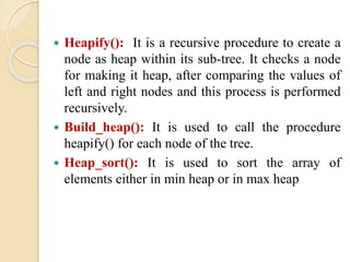
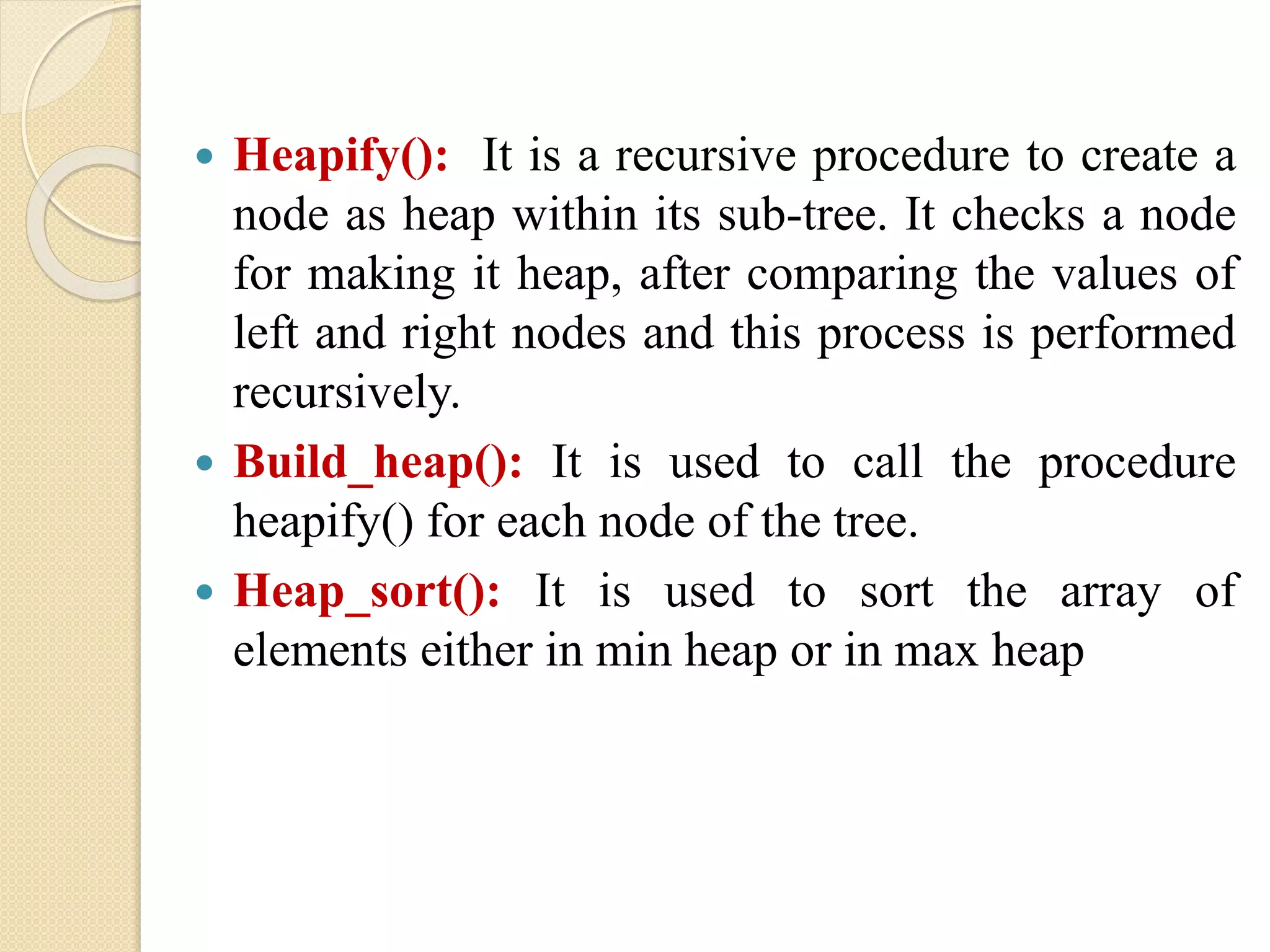
Heapify(): Itis a recursive procedure to create a
node as heap within its sub-tree. It checks a node
for making it heap, after comparing the values of
left and right nodes and this process is performed
recursively.
Build_heap(): It is used to call the procedure
heapify() for each node of the tree.
Heap_sort(): It is used to sort the array of
elements either in min heap or in max heap
41.
Algorithm Heapify():
Heapify()
Step1: Let L, R
Step 2: L = 2 * i + 1
Step 3: R = 2 * i + 2
Step 4: if (L < = length AND A[L] > A[i]) then Largest = L
Step 5: else Largest = I
[End of if]
Step 6:if (R < = length AND A[R] > A[Largest]) then Largest = R
[End of if]
Step 7: if(Largest != i) then
Temp = A[i]
A[i] = A[Largest]
A[largest] = Temp
Call Heapify(A, Largest)
[End of if]
Step 8: Exit
Algorithm Heap_sort():
Heap_sort(A)
Step1: Let Length = N - 1
Step 2: Call Build_heap(A)
Step 3: Repeat for I = Length to 1 decreasing by 1
Temp = A[i]
A[i] = A[0]
A[0] = Temp
Length = Length – 1
Call Heapify(A, 0)
[End of for]
Step 4: Exit
44.
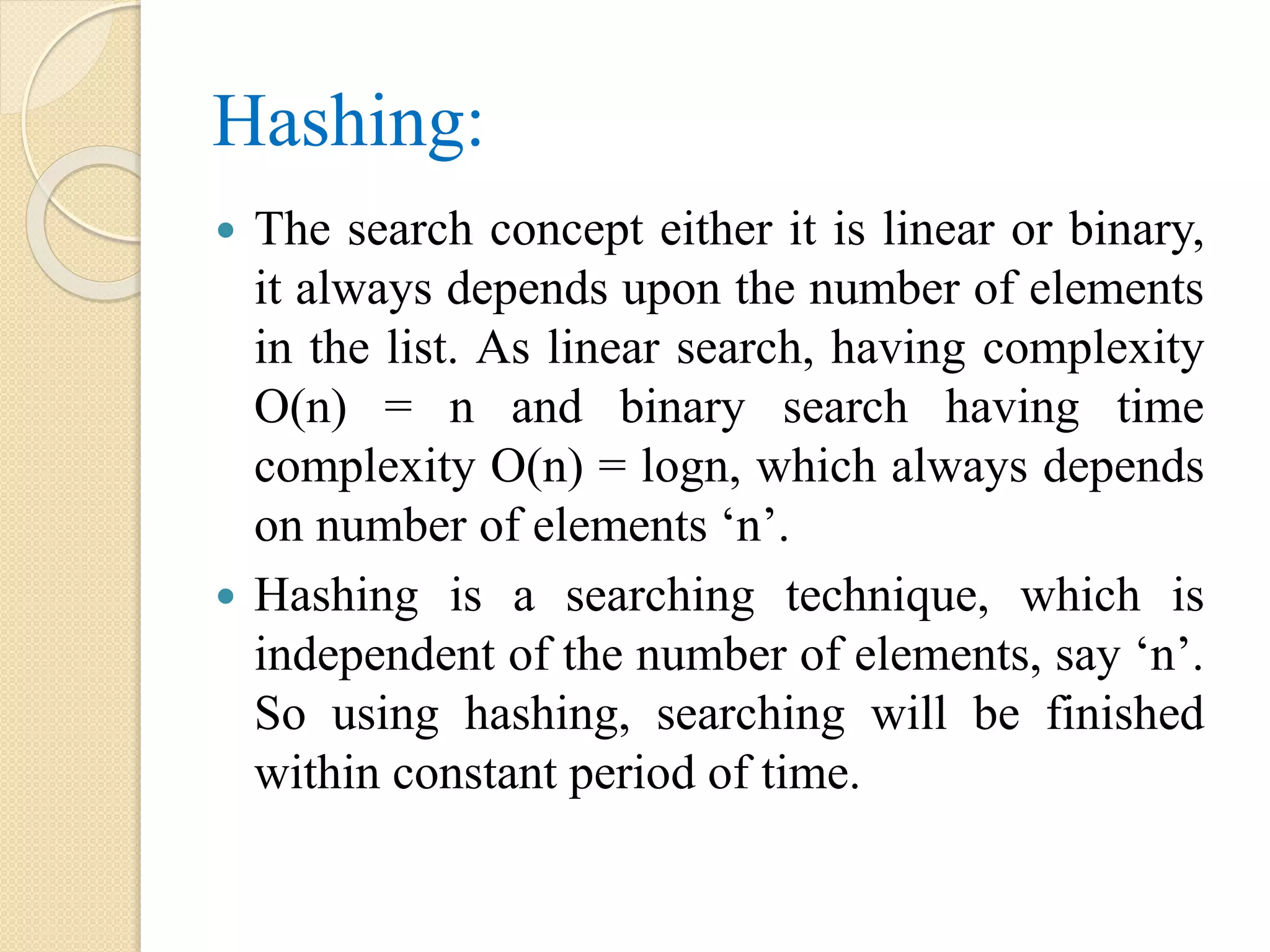
Hashing:
The searchconcept either it is linear or binary,
it always depends upon the number of elements
in the list. As linear search, having complexity
O(n) = n and binary search having time
complexity O(n) = logn, which always depends
on number of elements ‘n’.
Hashing is a searching technique, which is
independent of the number of elements, say ‘n’.
So using hashing, searching will be finished
within constant period of time.
45.
Hash Table:
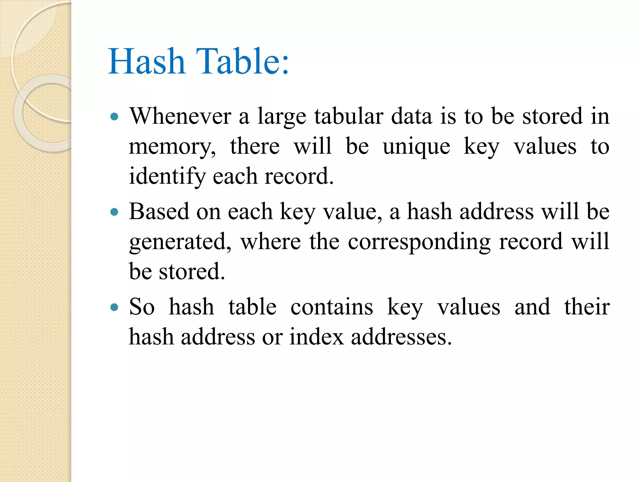
Whenevera large tabular data is to be stored in
memory, there will be unique key values to
identify each record.
Based on each key value, a hash address will be
generated, where the corresponding record will
be stored.
So hash table contains key values and their
hash address or index addresses.
46.
Hash Functions:
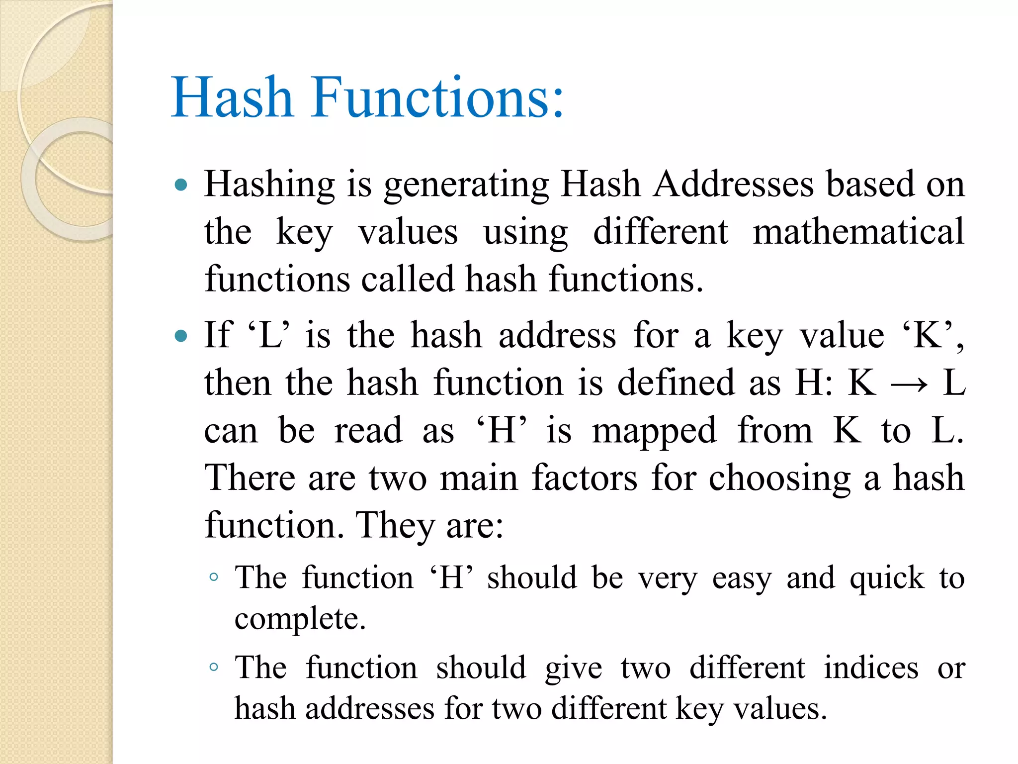
Hashingis generating Hash Addresses based on
the key values using different mathematical
functions called hash functions.
If ‘L’ is the hash address for a key value ‘K’,
then the hash function is defined as H: K → L
can be read as ‘H’ is mapped from K to L.
There are two main factors for choosing a hash
function. They are:
◦ The function ‘H’ should be very easy and quick to
complete.
◦ The function should give two different indices or
hash addresses for two different key values.
47.
Example:
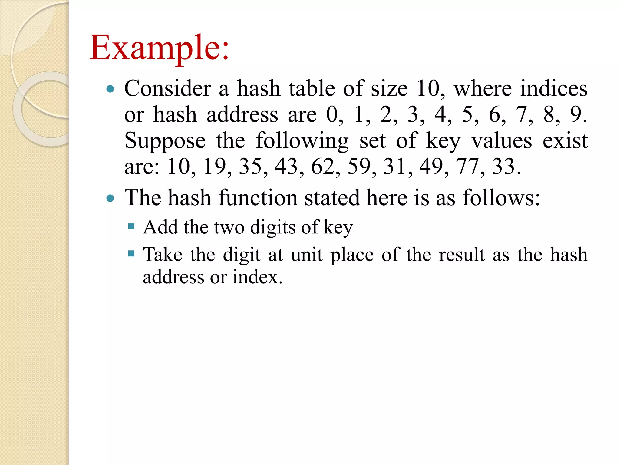
Consider ahash table of size 10, where indices
or hash address are 0, 1, 2, 3, 4, 5, 6, 7, 8, 9.
Suppose the following set of key values exist
are: 10, 19, 35, 43, 62, 59, 31, 49, 77, 33.
The hash function stated here is as follows:
Add the two digits of key
Take the digit at unit place of the result as the hash
address or index.
48.
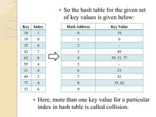
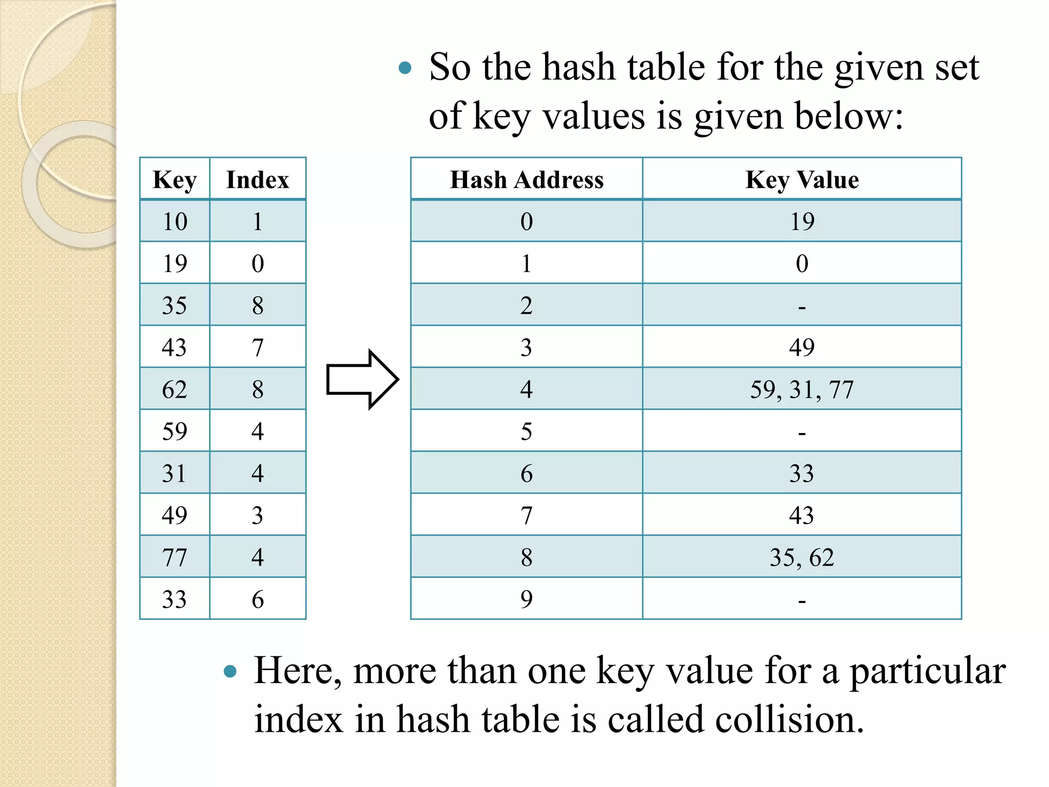
So thehash table for the given set
of key values is given below:
Key Index
10 1
19 0
35 8
43 7
62 8
59 4
31 4
49 3
77 4
33 6
Hash Address Key Value
0 19
1 0
2 -
3 49
4 59, 31, 77
5 -
6 33
7 43
8 35, 62
9 -
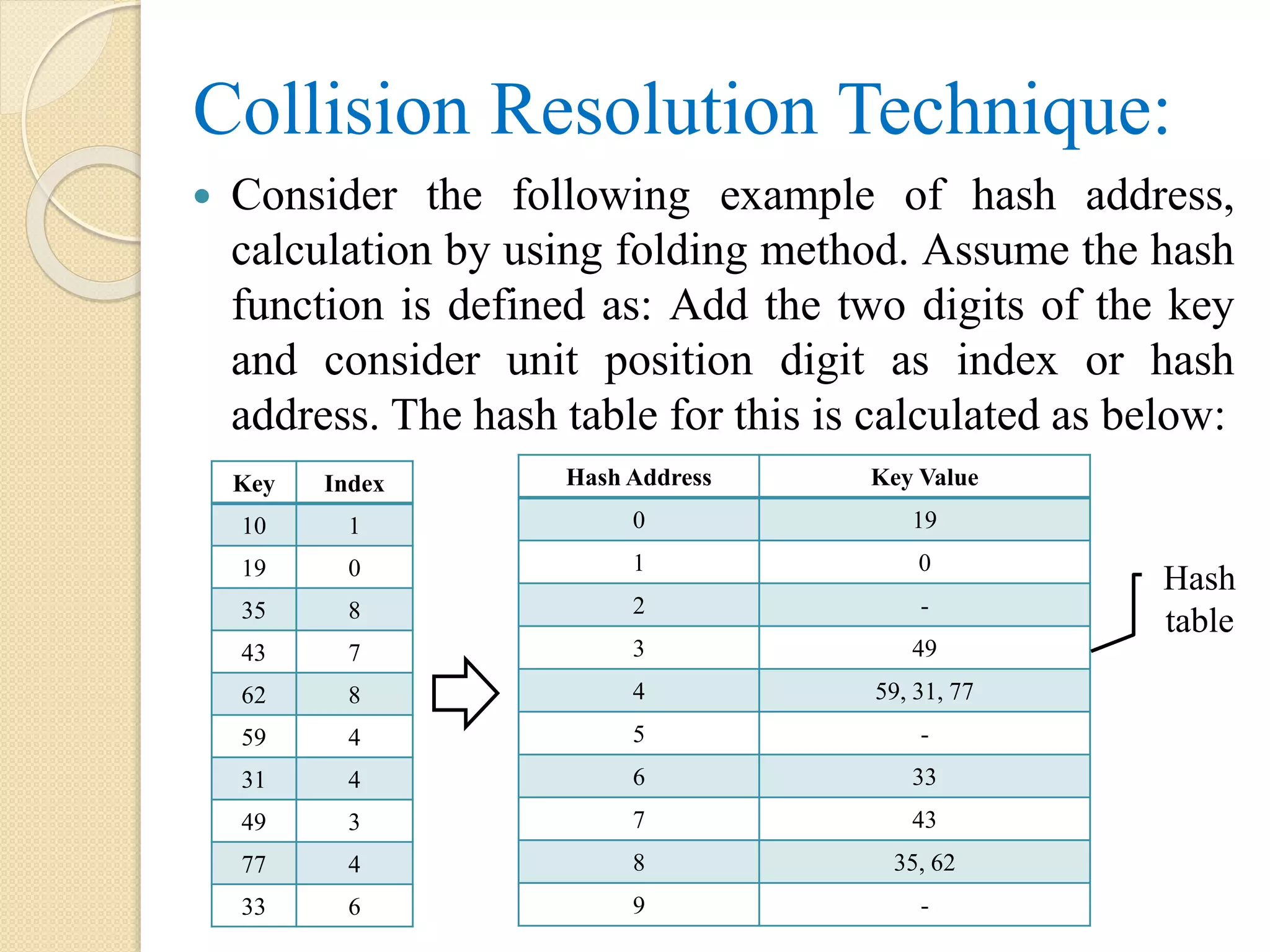
Here, more than one key value for a particular
index in hash table is called collision.
49.
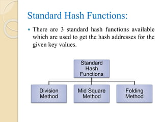
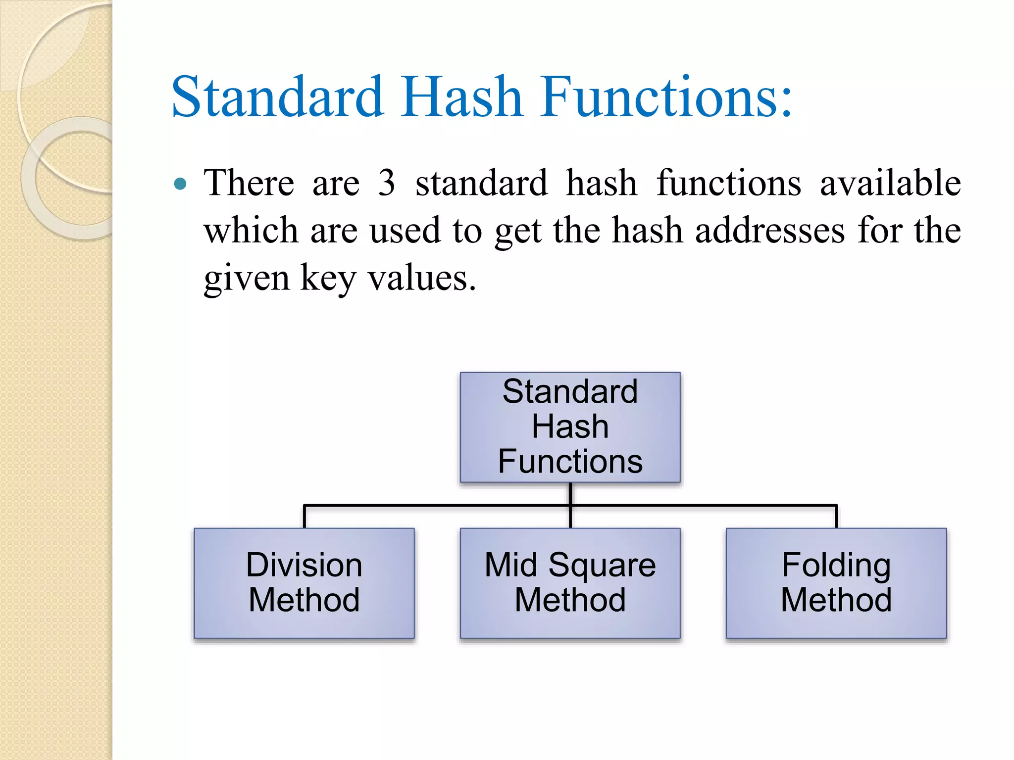
Standard Hash Functions:
There are 3 standard hash functions available
which are used to get the hash addresses for the
given key values.
Standard
Hash
Functions
Division
Method
Mid Square
Method
Folding
Method
50.
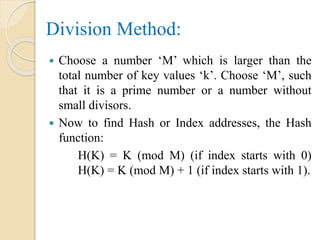
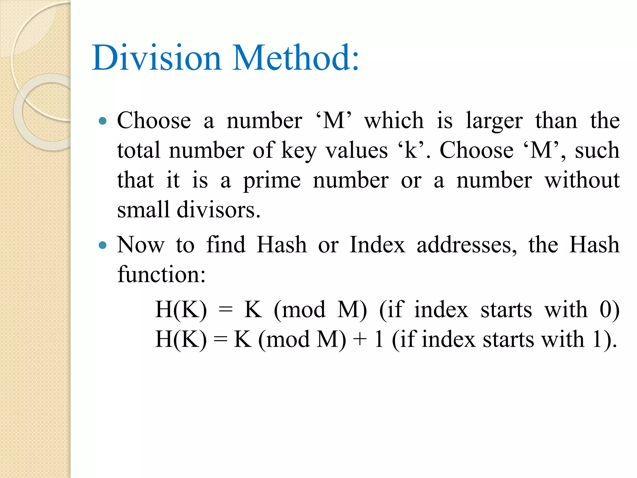
Division Method:
Choosea number ‘M’ which is larger than the
total number of key values ‘k’. Choose ‘M’, such
that it is a prime number or a number without
small divisors.
Now to find Hash or Index addresses, the Hash
function:
H(K) = K (mod M) (if index starts with 0)
H(K) = K (mod M) + 1 (if index starts with 1).
51.
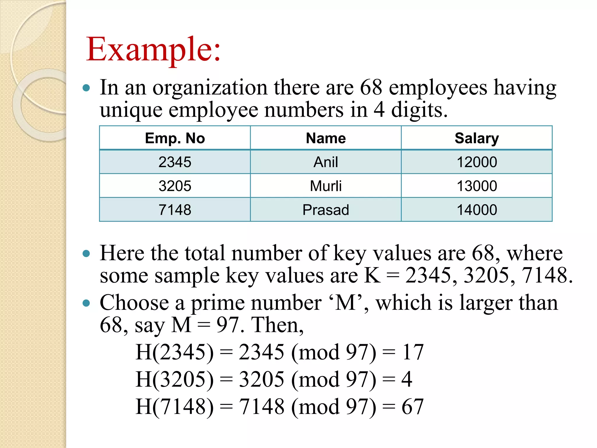
Example:
In anorganization there are 68 employees having
unique employee numbers in 4 digits.
Here the total number of key values are 68, where
some sample key values are K = 2345, 3205, 7148.
Choose a prime number ‘M’, which is larger than
68, say M = 97. Then,
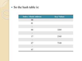
H(2345) = 2345 (mod 97) = 17
H(3205) = 3205 (mod 97) = 4
H(7148) = 7148 (mod 97) = 67
Emp. No Name Salary
2345 Anil 12000
3205 Murli 13000
7148 Prasad 14000
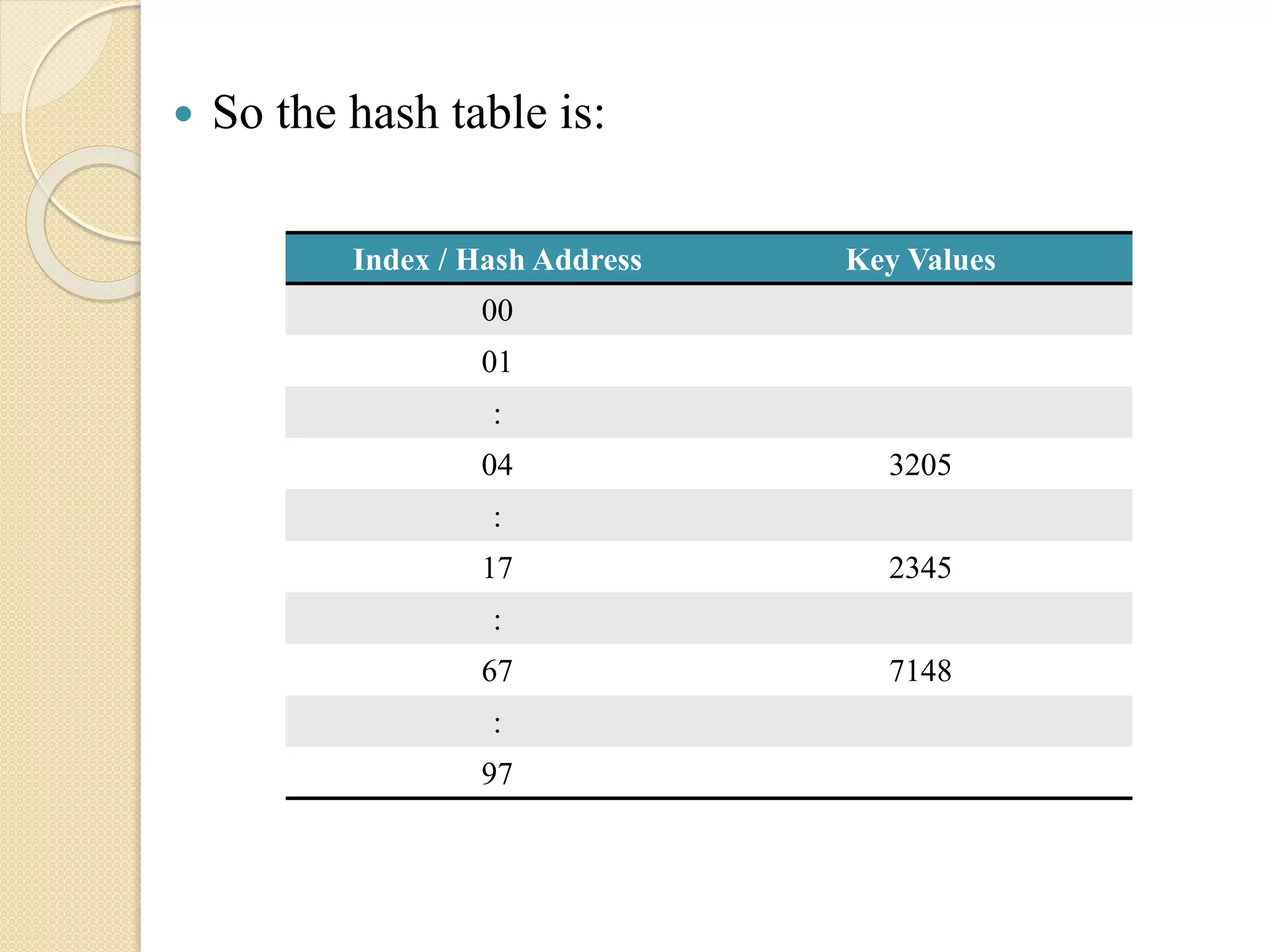
52.
So thehash table is:
Index / Hash Address Key Values
00
01
:
04 3205
:
17 2345
:
67 7148
:
97
53.
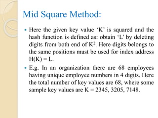
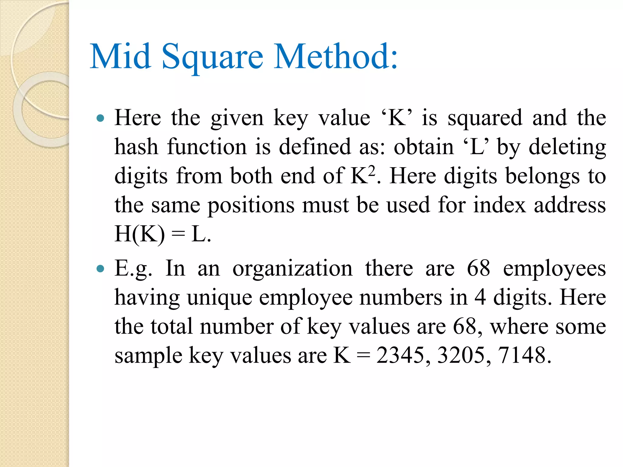
Mid Square Method:
Here the given key value ‘K’ is squared and the
hash function is defined as: obtain ‘L’ by deleting
digits from both end of K2. Here digits belongs to
the same positions must be used for index address
H(K) = L.
E.g. In an organization there are 68 employees
having unique employee numbers in 4 digits. Here
the total number of key values are 68, where some
sample key values are K = 2345, 3205, 7148.
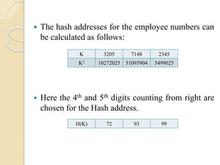
54.
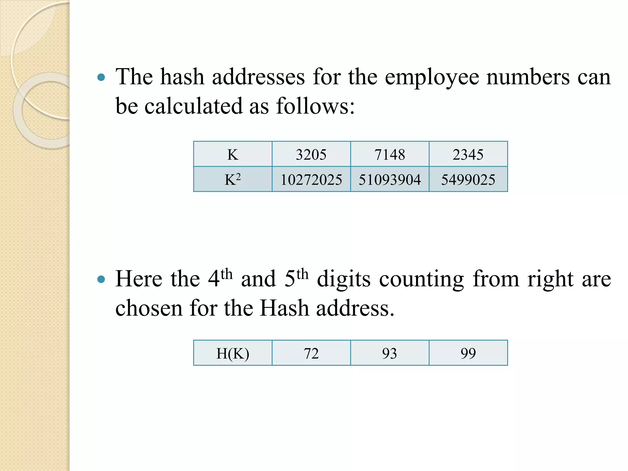
The hashaddresses for the employee numbers can
be calculated as follows:
Here the 4th and 5th digits counting from right are
chosen for the Hash address.
K 3205 7148 2345
K2 10272025 51093904 5499025
H(K) 72 93 99
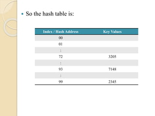
55.
So thehash table is:
Index / Hash Address Key Values
00
01
:
72 3205
:
93 7148
:
99 2345
56.
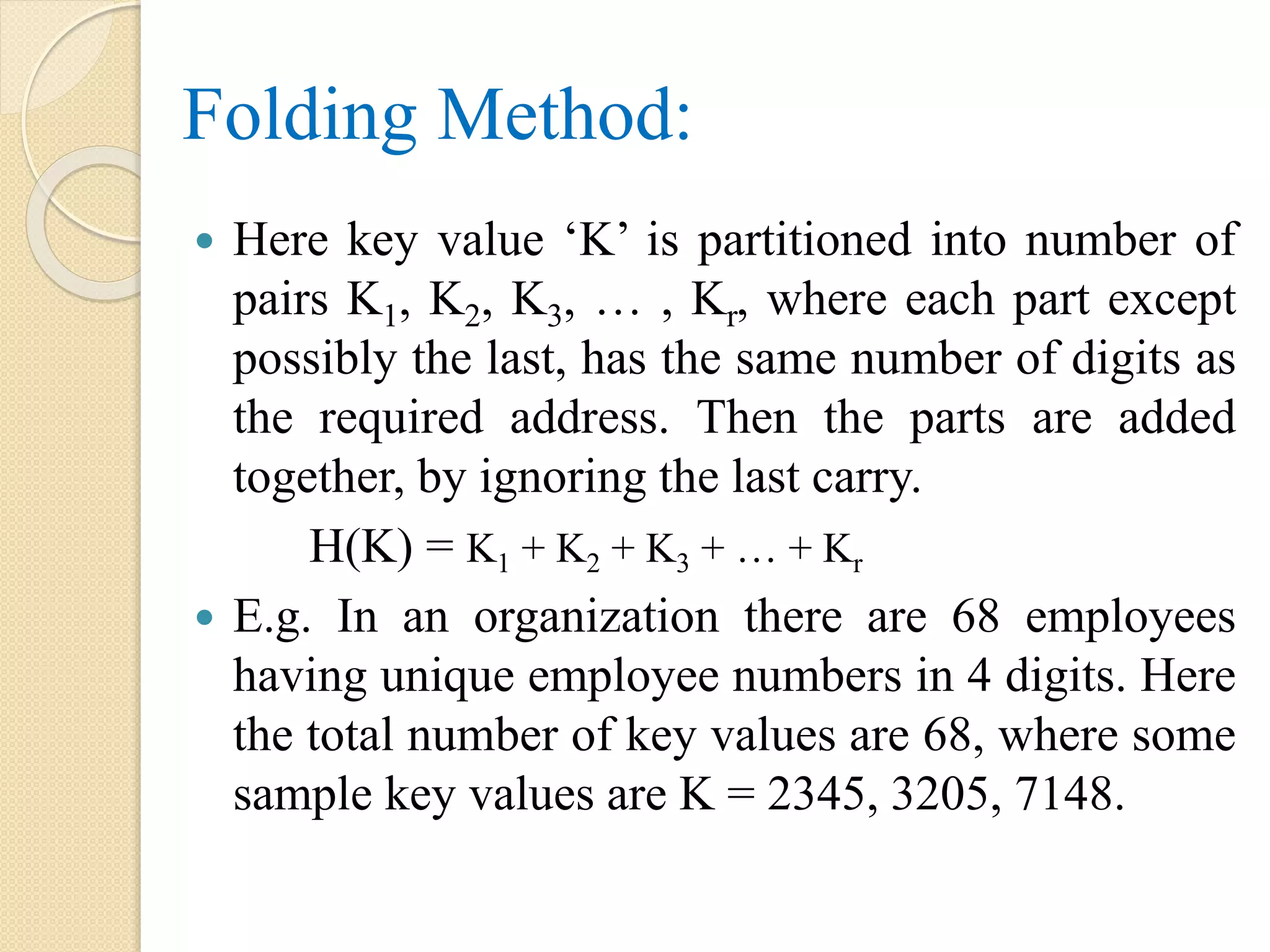
Folding Method:
Herekey value ‘K’ is partitioned into number of
pairs K1, K2, K3, … , Kr, where each part except
possibly the last, has the same number of digits as
the required address. Then the parts are added
together, by ignoring the last carry.
H(K) = K1 + K2 + K3 + … + Kr
E.g. In an organization there are 68 employees
having unique employee numbers in 4 digits. Here
the total number of key values are 68, where some
sample key values are K = 2345, 3205, 7148.
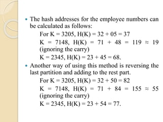
57.
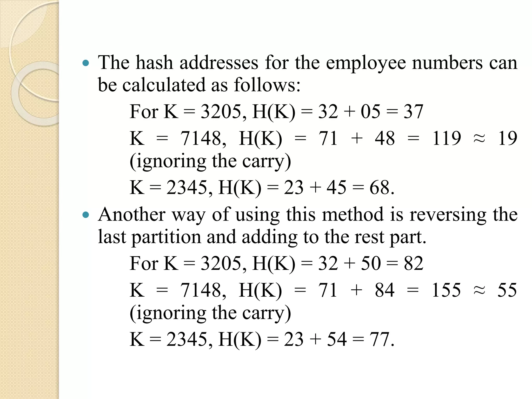
The hashaddresses for the employee numbers can
be calculated as follows:
For K = 3205, H(K) = 32 + 05 = 37
K = 7148, H(K) = 71 + 48 = 119 ≈ 19
(ignoring the carry)
K = 2345, H(K) = 23 + 45 = 68.
Another way of using this method is reversing the
last partition and adding to the rest part.
For K = 3205, H(K) = 32 + 50 = 82
K = 7148, H(K) = 71 + 84 = 155 ≈ 55
(ignoring the carry)
K = 2345, H(K) = 23 + 54 = 77.
58.
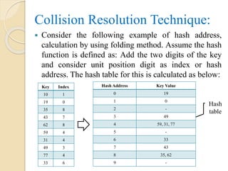
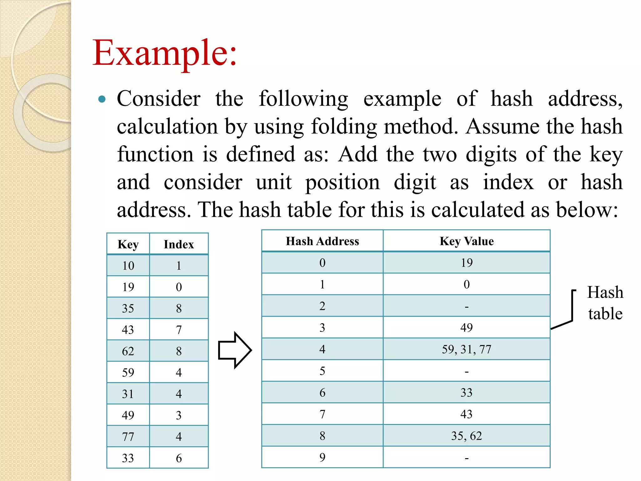
Collision Resolution Technique:
Consider the following example of hash address,
calculation by using folding method. Assume the hash
function is defined as: Add the two digits of the key
and consider unit position digit as index or hash
address. The hash table for this is calculated as below:
Key Index
10 1
19 0
35 8
43 7
62 8
59 4
31 4
49 3
77 4
33 6
Hash Address Key Value
0 19
1 0
2 -
3 49
4 59, 31, 77
5 -
6 33
7 43
8 35, 62
9 -
Hash
table
59.
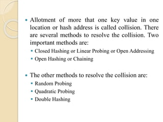
Allotment ofmore that one key value in one
location or hash address is called collision. There
are several methods to resolve the collision. Two
important methods are:
Closed Hashing or Linear Probing or Open Addressing
Open Hashing or Chaining
The other methods to resolve the collision are:
Random Probing
Quadratic Probing
Double Hashing
60.
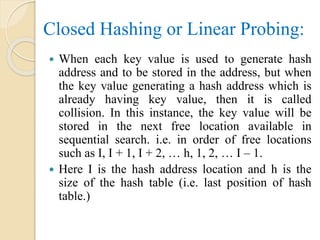
Closed Hashing orLinear Probing:
When each key value is used to generate hash
address and to be stored in the address, but when
the key value generating a hash address which is
already having key value, then it is called
collision. In this instance, the key value will be
stored in the next free location available in
sequential search. i.e. in order of free locations
such as I, I + 1, I + 2, … h, 1, 2, … I – 1.
Here I is the hash address location and h is the
size of the hash table (i.e. last position of hash
table.)
61.
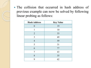
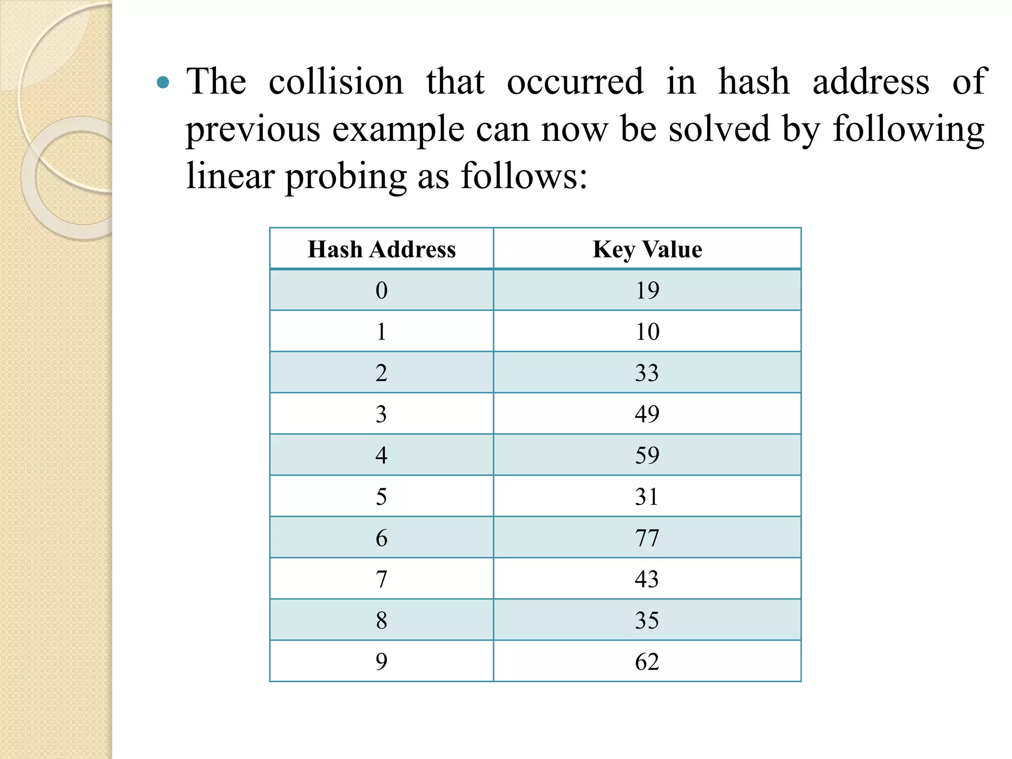
The collisionthat occurred in hash address of
previous example can now be solved by following
linear probing as follows:
Hash Address Key Value
0 19
1 10
2 33
3 49
4 59
5 31
6 77
7 43
8 35
9 62
62.
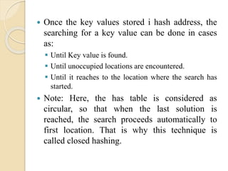
Once thekey values stored i hash address, the
searching for a key value can be done in cases
as:
Until Key value is found.
Until unoccupied locations are encountered.
Until it reaches to the location where the search has
started.
Note: Here, the has table is considered as
circular, so that when the last solution is
reached, the search proceeds automatically to
first location. That is why this technique is
called closed hashing.
63.
Drawbacks of ClosedHashing:
When more number of collisions occurs, the
sequential search increases and search will
become slow.
It is difficult to handle the overflow situation of
hash table is satisfactory manner.
Key values are haphazardly intermixed due to
more probing.
64.
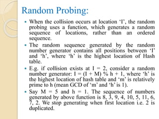
Random Probing:
Whenthe collision occurs at location ‘I’, the random
probing uses a function, which generates a random
sequence of locations, rather than an ordered
sequence.
The random sequence generated by the random
number generator contains all positions between ‘I’
and ‘h’, where ‘h’ is the highest location of Hash
table.
E.g. if collision exists at I = 2, consider a random
number generator: I = (I + M) % h + 1, where ‘h’ is
the highest location of hash table and ‘m’ is relatively
prime to h (mean GCD of ‘m’ and ‘h’ is 1).
Say M = 5 and h = 1. The sequence of numbers
generated by above function is 8, 3, 9, 4, 10, 5, 11, 6,
7, 2. We stop generating when first location i.e. 2 is
duplicated.
65.
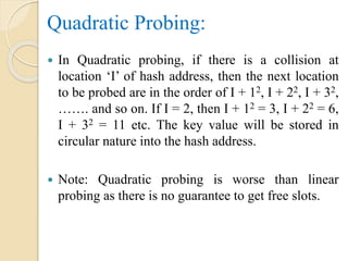
Quadratic Probing:
InQuadratic probing, if there is a collision at
location ‘I’ of hash address, then the next location
to be probed are in the order of I + 12, I + 22, I + 32,
……. and so on. If I = 2, then I + 12 = 3, I + 22 = 6,
I + 32 = 11 etc. The key value will be stored in
circular nature into the hash address.
Note: Quadratic probing is worse than linear
probing as there is no guarantee to get free slots.
66.
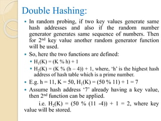
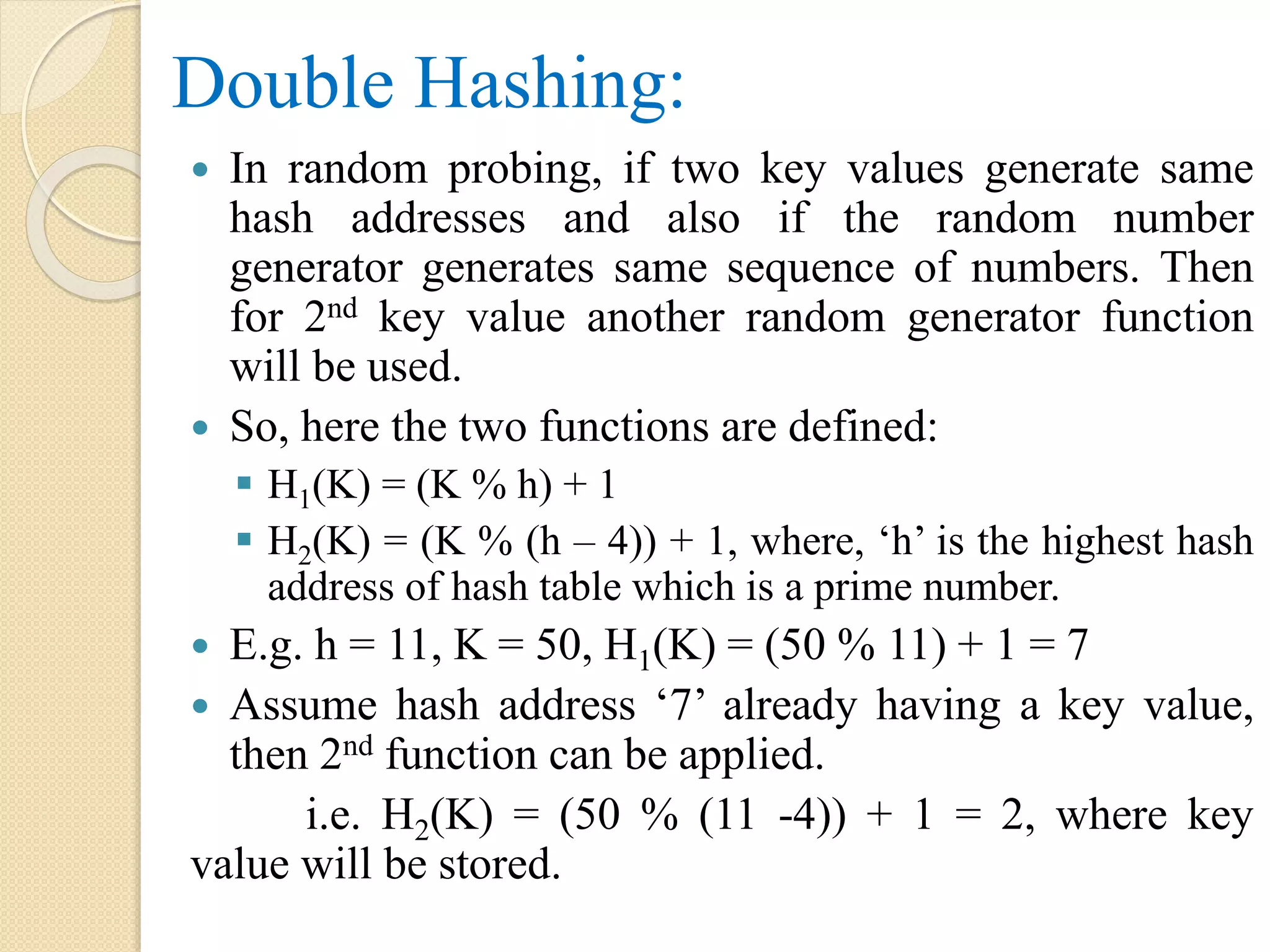
Double Hashing:
Inrandom probing, if two key values generate same
hash addresses and also if the random number
generator generates same sequence of numbers. Then
for 2nd key value another random generator function
will be used.
So, here the two functions are defined:
H1(K) = (K % h) + 1
H2(K) = (K % (h – 4)) + 1, where, ‘h’ is the highest hash
address of hash table which is a prime number.
E.g. h = 11, K = 50, H1(K) = (50 % 11) + 1 = 7
Assume hash address ‘7’ already having a key value,
then 2nd function can be applied.
i.e. H2(K) = (50 % (11 -4)) + 1 = 2, where key
value will be stored.
67.
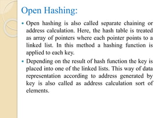
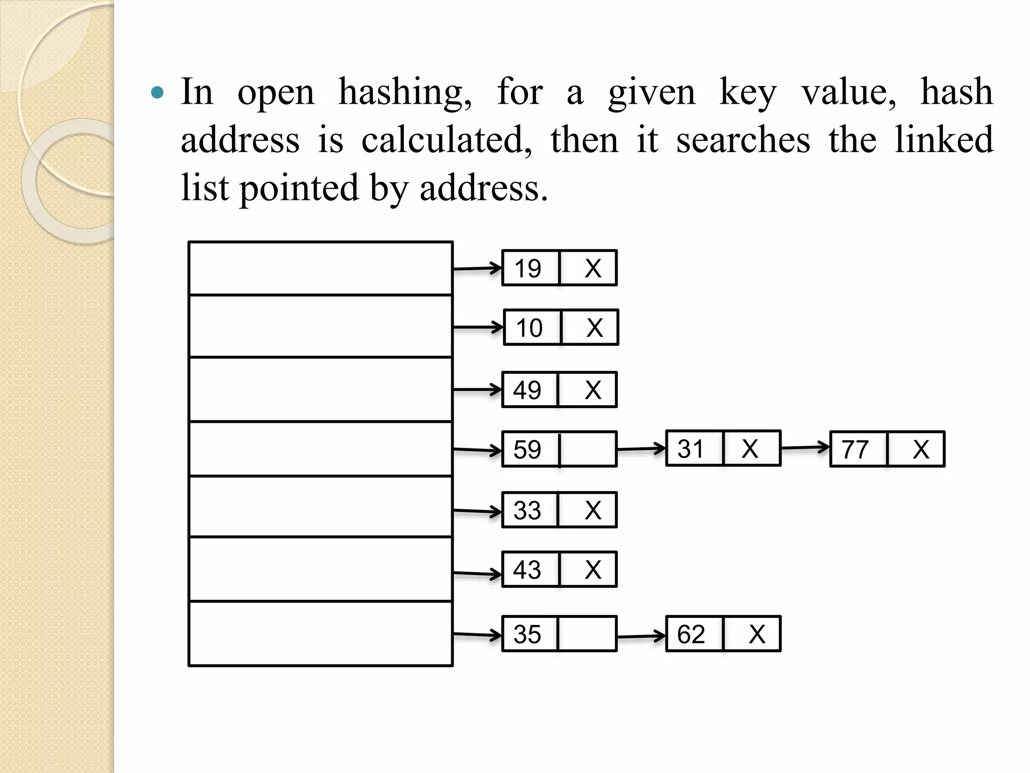
Open Hashing:
Openhashing is also called separate chaining or
address calculation. Here, the hash table is treated
as array of pointers where each pointer points to a
linked list. In this method a hashing function is
applied to each key.
Depending on the result of hash function the key is
placed into one of the linked lists. This way of data
representation according to address generated by
key is also called as address calculation sort of
elements.
68.
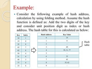
Example:
Consider thefollowing example of hash address,
calculation by using folding method. Assume the hash
function is defined as: Add the two digits of the key
and consider unit position digit as index or hash
address. The hash table for this is calculated as below:
Key Index
10 1
19 0
35 8
43 7
62 8
59 4
31 4
49 3
77 4
33 6
Hash Address Key Value
0 19
1 0
2 -
3 49
4 59, 31, 77
5 -
6 33
7 43
8 35, 62
9 -
Hash
table
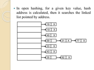
69.
In openhashing, for a given key value, hash
address is calculated, then it searches the linked
list pointed by address.
19 X
10 X
49 X
59 77 X31 X
33 X
43 X
62 X35
70.
Advantages of Chaining:
Overflow situation don’t arise in hash table.
Collision resolution can be easily achieved by
maintaining linked list in memory.
Insertion and deletion becomes easy and it is best
than closed hashing.
End
![Algorithm:
LinearSearch(LA, LB, UB, ITEM)
Step 1: Let K, FLAG
Step 2: Set K = LB, FLAG = 0
Step 3: Repeat while(K <= UB)
Step 3.1: if LA[K] = ITEM, then
Step 3.1.1: Set FLAG = 1
Step 3.1.2: Display “ITEM found at”, K
[End of if]
Step 3.2: Set K = K + 1
[End of while]
Step 4: if FLAG = 0, then
Step 4.1: Display “ITEM is not found”.
[End of if]
Step 5: Exit
Note: Here,
linear
array(LA)
upper bound
(UB)
lower bound
(LB)](https://image.slidesharecdn.com/datastructureusingcmodule3-170522041907/85/Data-structure-using-c-module-3-5-320.jpg)
![Algorithm:
BinarySearch(LA, LB, UB, ITEM)
Step 1: Let BEG, END, MID, LOC
Step 2: Set BEG = LB, END = UB,
MID = (BEG + END)/2
Step 3: Repeat,
while BEG <= END AND LA[MID] != ITEM
Step 3.1: if ITEM < LA[MID], then set END = MID - 1
Step 3.2: else set BEG = MID + 1
[End of if]
Step 3.3: Set MID = ( BEG + END)/2
[End of while Step 3]
Step 4: if LA[MID] = ITEM, then set LOC = MID
else
set LOC = 0
[End of if]
Step 5: Exit](https://image.slidesharecdn.com/datastructureusingcmodule3-170522041907/85/Data-structure-using-c-module-3-7-320.jpg)
![Algorithm:
Selection_Sort(A[N])
Step 1: Let I, J, TEMP
Step 2: Repeat for I = 0 to N – 1 increasing by 1
Step 2.1: Repeat for J = I + 1 to N increasing by 1
Step 2.1.1: if A[I] > A[J], then
TEMP = A[I]
A[I] = A[J]
A[J] = TEMP
[End of if]
[End of for]
[End of for]
Step 3: Exit](https://image.slidesharecdn.com/datastructureusingcmodule3-170522041907/85/Data-structure-using-c-module-3-12-320.jpg)

![Algorithm:
Step 1: Let I, K, TEMP
Step 2: Repeat for K = N-2 to 0 decreasing by 1
Step 2.1: Repeat for I = 0 to K increasing by 1
Step 2.1.1: if A[I] > A[I + 1], then
TEMP = A[I]
A[I] = A[I + 1]
A[I + 1] = TEMP
[End of if]
[End of for]
[End of for]
Step 3: Exit](https://image.slidesharecdn.com/datastructureusingcmodule3-170522041907/85/Data-structure-using-c-module-3-15-320.jpg)
![Algorithm:
Insertion_Sort(A[N])
Step 1: Let J, K, TEMP
Step 2: Set K = 1
Step 3: Repeat for K = 1 to N – 1 increasing by 1
Set TEMP = A[K]
J = K - 1
Step 3.1: Repeat while ((J >= 0) AND (TEMP < A[J]))
A[J + 1] = A[J]
J = J - 1
[End of while]
Step 3.2: A[J + 1] = TEMP
[End of for]
Step 4: Exit](https://image.slidesharecdn.com/datastructureusingcmodule3-170522041907/85/Data-structure-using-c-module-3-21-320.jpg)
![Algorithm:
Step 1: Set Large = largest element of the Array
Step 2: Set Num = total number of digits in Large
Step 3: Repeat for Pass = 1 to Num by 1
Step 3.1: Initialize all buckets (0 to 9)
Step 3.2: Repeat for I = 0 to N – 1 by 1
Step 3.2.1: Set Digit = obtain digit at Pass – 1 position
of A[I]
Step 3.2.2: Put A[I] into the bucket Digit
[End of for – Step 3.2]
Step 3.3: Recollect numbers from buckets from 0 to 9
into array A
[End of for – Step 3]
Step 4: Exit](https://image.slidesharecdn.com/datastructureusingcmodule3-170522041907/85/Data-structure-using-c-module-3-26-320.jpg)


![Algorithm: Merge
Merge (A, p, q, r)
Step 1: n1 ← q – p + 1
Step 2: n2 ← r - q
Step 3: create arrays L[1…n1 + 1] and R[1…n2 + 1]
Step 4: for i ← 1 to n1
Step 5: do L[i] ← A[p + i – 1]
Step 6: for j ← 1 to n2
Step 7: do R[j] ← A[q + j]
Step 8: L[n1 + 1] ← ∞
Step 9: R[n2 + 1] ← ∞
Step 10: i ← 1](https://image.slidesharecdn.com/datastructureusingcmodule3-170522041907/85/Data-structure-using-c-module-3-33-320.jpg)
![ Step 11: j ← 1
Step 12: for k ← p to r
Step 13: do if L[i] ≤ R[j]
Step 14: then A[k] ← L[i]
Step 15: i ← i + 1
Step 16: else A[k] ← R[j]
Step 17: j ← j + 1
Time complexity of Merge Sort:
The time complexity of Merge Sort (total time) is:
T(n) = θ(nlogn) and total cost = cnlogn.
Merge procedure on an ‘n’ elements sub-array
takes time θ(n).](https://image.slidesharecdn.com/datastructureusingcmodule3-170522041907/85/Data-structure-using-c-module-3-34-320.jpg)
![Algorithm: Partition
Partition(A, p, r)
Step 1: x ← A[r]
Step 2: i ← p - 1
Step 3: j ← p to r - 1
Step 4: do if A[j] ≤ x
Step 5: then i ← i + 1
Step 6: exchange A[i] ↔ A[j]
Step 7: exchange A[i + 1] ↔ A[r]
Step 8: return](https://image.slidesharecdn.com/datastructureusingcmodule3-170522041907/85/Data-structure-using-c-module-3-39-320.jpg)
![Algorithm Heapify():
Heapify()
Step 1: Let L, R
Step 2: L = 2 * i + 1
Step 3: R = 2 * i + 2
Step 4: if (L < = length AND A[L] > A[i]) then Largest = L
Step 5: else Largest = I
[End of if]
Step 6:if (R < = length AND A[R] > A[Largest]) then Largest = R
[End of if]
Step 7: if(Largest != i) then
Temp = A[i]
A[i] = A[Largest]
A[largest] = Temp
Call Heapify(A, Largest)
[End of if]
Step 8: Exit](https://image.slidesharecdn.com/datastructureusingcmodule3-170522041907/85/Data-structure-using-c-module-3-41-320.jpg)
![Algorithm Build_heap():
Build_heap(A)
Step 1: Let I = (N / 2) - 1
Step 2: Repeat while(I > = 0)
Call Heapify(A, I)
I = I – 1
[End of while]
Step 3: Exit](https://image.slidesharecdn.com/datastructureusingcmodule3-170522041907/85/Data-structure-using-c-module-3-42-320.jpg)
![Algorithm Heap_sort():
Heap_sort(A)
Step 1: Let Length = N - 1
Step 2: Call Build_heap(A)
Step 3: Repeat for I = Length to 1 decreasing by 1
Temp = A[i]
A[i] = A[0]
A[0] = Temp
Length = Length – 1
Call Heapify(A, 0)
[End of for]
Step 4: Exit](https://image.slidesharecdn.com/datastructureusingcmodule3-170522041907/85/Data-structure-using-c-module-3-43-320.jpg)


![Algorithm:
LinearSearch(LA, LB, UB, ITEM)
Step 1: Let K, FLAG
Step 2: Set K = LB, FLAG = 0
Step 3: Repeat while(K <= UB)
Step 3.1: if LA[K] = ITEM, then
Step 3.1.1: Set FLAG = 1
Step 3.1.2: Display “ITEM found at”, K
[End of if]
Step 3.2: Set K = K + 1
[End of while]
Step 4: if FLAG = 0, then
Step 4.1: Display “ITEM is not found”.
[End of if]
Step 5: Exit
Note: Here,
linear
array(LA)
upper bound
(UB)
lower bound
(LB)](https://image.slidesharecdn.com/datastructureusingcmodule3-170522041907/75/Data-structure-using-c-module-3-5-2048.jpg)
![Algorithm:
BinarySearch(LA, LB, UB, ITEM)
Step 1: Let BEG, END, MID, LOC
Step 2: Set BEG = LB, END = UB,
MID = (BEG + END)/2
Step 3: Repeat,
while BEG <= END AND LA[MID] != ITEM
Step 3.1: if ITEM < LA[MID], then set END = MID - 1
Step 3.2: else set BEG = MID + 1
[End of if]
Step 3.3: Set MID = ( BEG + END)/2
[End of while Step 3]
Step 4: if LA[MID] = ITEM, then set LOC = MID
else
set LOC = 0
[End of if]
Step 5: Exit](https://image.slidesharecdn.com/datastructureusingcmodule3-170522041907/75/Data-structure-using-c-module-3-7-2048.jpg)
![Algorithm:
Selection_Sort(A[N])
Step 1: Let I, J, TEMP
Step 2: Repeat for I = 0 to N – 1 increasing by 1
Step 2.1: Repeat for J = I + 1 to N increasing by 1
Step 2.1.1: if A[I] > A[J], then
TEMP = A[I]
A[I] = A[J]
A[J] = TEMP
[End of if]
[End of for]
[End of for]
Step 3: Exit](https://image.slidesharecdn.com/datastructureusingcmodule3-170522041907/75/Data-structure-using-c-module-3-12-2048.jpg)
![Algorithm:
Step 1: Let I, K, TEMP
Step 2: Repeat for K = N-2 to 0 decreasing by 1
Step 2.1: Repeat for I = 0 to K increasing by 1
Step 2.1.1: if A[I] > A[I + 1], then
TEMP = A[I]
A[I] = A[I + 1]
A[I + 1] = TEMP
[End of if]
[End of for]
[End of for]
Step 3: Exit](https://image.slidesharecdn.com/datastructureusingcmodule3-170522041907/75/Data-structure-using-c-module-3-15-2048.jpg)
![Algorithm:
Insertion_Sort(A[N])
Step 1: Let J, K, TEMP
Step 2: Set K = 1
Step 3: Repeat for K = 1 to N – 1 increasing by 1
Set TEMP = A[K]
J = K - 1
Step 3.1: Repeat while ((J >= 0) AND (TEMP < A[J]))
A[J + 1] = A[J]
J = J - 1
[End of while]
Step 3.2: A[J + 1] = TEMP
[End of for]
Step 4: Exit](https://image.slidesharecdn.com/datastructureusingcmodule3-170522041907/75/Data-structure-using-c-module-3-21-2048.jpg)
![Algorithm:
Step 1: Set Large = largest element of the Array
Step 2: Set Num = total number of digits in Large
Step 3: Repeat for Pass = 1 to Num by 1
Step 3.1: Initialize all buckets (0 to 9)
Step 3.2: Repeat for I = 0 to N – 1 by 1
Step 3.2.1: Set Digit = obtain digit at Pass – 1 position
of A[I]
Step 3.2.2: Put A[I] into the bucket Digit
[End of for – Step 3.2]
Step 3.3: Recollect numbers from buckets from 0 to 9
into array A
[End of for – Step 3]
Step 4: Exit](https://image.slidesharecdn.com/datastructureusingcmodule3-170522041907/75/Data-structure-using-c-module-3-26-2048.jpg)
![Algorithm: Merge
Merge (A, p, q, r)
Step 1: n1 ← q – p + 1
Step 2: n2 ← r - q
Step 3: create arrays L[1…n1 + 1] and R[1…n2 + 1]
Step 4: for i ← 1 to n1
Step 5: do L[i] ← A[p + i – 1]
Step 6: for j ← 1 to n2
Step 7: do R[j] ← A[q + j]
Step 8: L[n1 + 1] ← ∞
Step 9: R[n2 + 1] ← ∞
Step 10: i ← 1](https://image.slidesharecdn.com/datastructureusingcmodule3-170522041907/75/Data-structure-using-c-module-3-33-2048.jpg)
![ Step 11: j ← 1
Step 12: for k ← p to r
Step 13: do if L[i] ≤ R[j]
Step 14: then A[k] ← L[i]
Step 15: i ← i + 1
Step 16: else A[k] ← R[j]
Step 17: j ← j + 1
Time complexity of Merge Sort:
The time complexity of Merge Sort (total time) is:
T(n) = θ(nlogn) and total cost = cnlogn.
Merge procedure on an ‘n’ elements sub-array
takes time θ(n).](https://image.slidesharecdn.com/datastructureusingcmodule3-170522041907/75/Data-structure-using-c-module-3-34-2048.jpg)
![Algorithm: Partition
Partition(A, p, r)
Step 1: x ← A[r]
Step 2: i ← p - 1
Step 3: j ← p to r - 1
Step 4: do if A[j] ≤ x
Step 5: then i ← i + 1
Step 6: exchange A[i] ↔ A[j]
Step 7: exchange A[i + 1] ↔ A[r]
Step 8: return](https://image.slidesharecdn.com/datastructureusingcmodule3-170522041907/75/Data-structure-using-c-module-3-39-2048.jpg)
![Algorithm Heapify():
Heapify()
Step 1: Let L, R
Step 2: L = 2 * i + 1
Step 3: R = 2 * i + 2
Step 4: if (L < = length AND A[L] > A[i]) then Largest = L
Step 5: else Largest = I
[End of if]
Step 6:if (R < = length AND A[R] > A[Largest]) then Largest = R
[End of if]
Step 7: if(Largest != i) then
Temp = A[i]
A[i] = A[Largest]
A[largest] = Temp
Call Heapify(A, Largest)
[End of if]
Step 8: Exit](https://image.slidesharecdn.com/datastructureusingcmodule3-170522041907/75/Data-structure-using-c-module-3-41-2048.jpg)
![Algorithm Build_heap():
Build_heap(A)
Step 1: Let I = (N / 2) - 1
Step 2: Repeat while(I > = 0)
Call Heapify(A, I)
I = I – 1
[End of while]
Step 3: Exit](https://image.slidesharecdn.com/datastructureusingcmodule3-170522041907/75/Data-structure-using-c-module-3-42-2048.jpg)
![Algorithm Heap_sort():
Heap_sort(A)
Step 1: Let Length = N - 1
Step 2: Call Build_heap(A)
Step 3: Repeat for I = Length to 1 decreasing by 1
Temp = A[i]
A[i] = A[0]
A[0] = Temp
Length = Length – 1
Call Heapify(A, 0)
[End of for]
Step 4: Exit](https://image.slidesharecdn.com/datastructureusingcmodule3-170522041907/75/Data-structure-using-c-module-3-43-2048.jpg)


![UNIT V Searching Sorting Hashing Techniques [Autosaved].pptx](https://cdn.slidesharecdn.com/ss_thumbnails/unitvsearchingsortinghashingtechniquesautosaved-241014040608-74caa0f6-thumbnail.jpg?width=600ounds&width=560&fit=bounds)
![UNIT V Searching Sorting Hashing Techniques [Autosaved].pptx](https://cdn.slidesharecdn.com/ss_thumbnails/unitvsearchingsortinghashingtechniquesautosaved-241126054304-95a69c51-thumbnail.jpg?width=600ounds&width=560&fit=bounds)


