
![Induction Example:
Gaussian Closed Form
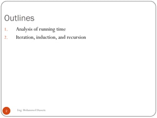
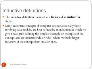
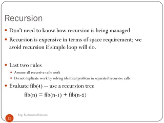
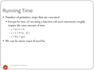
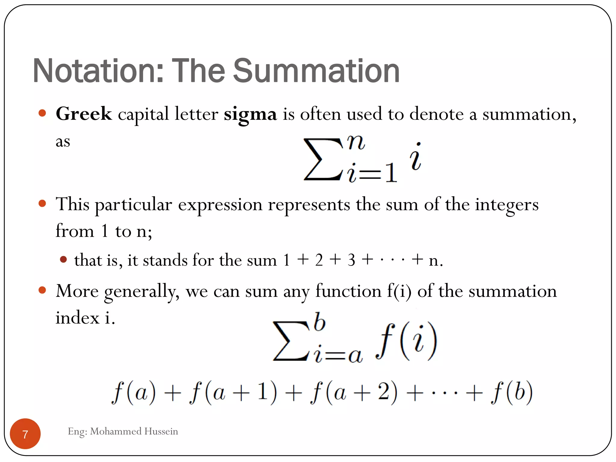
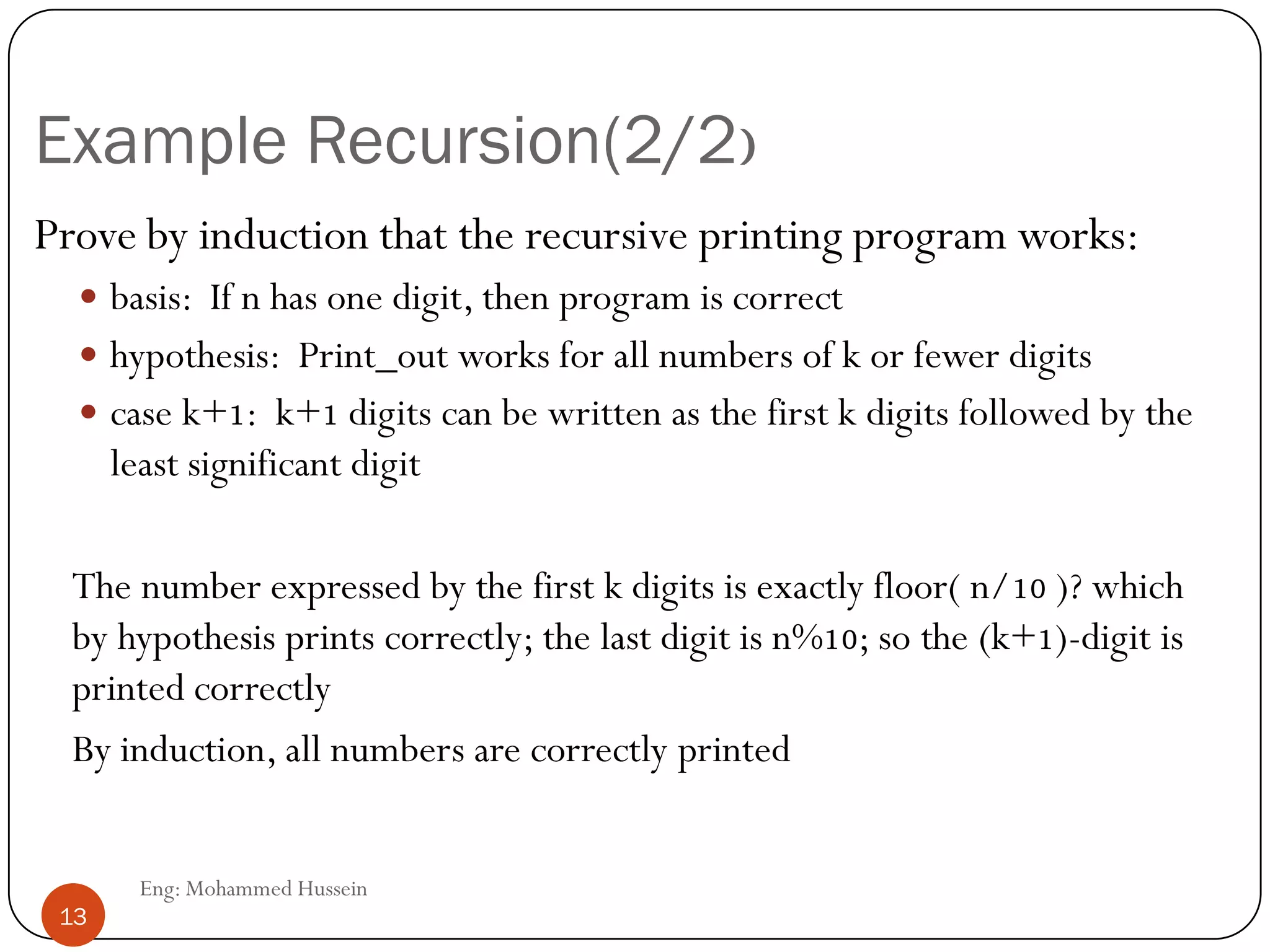
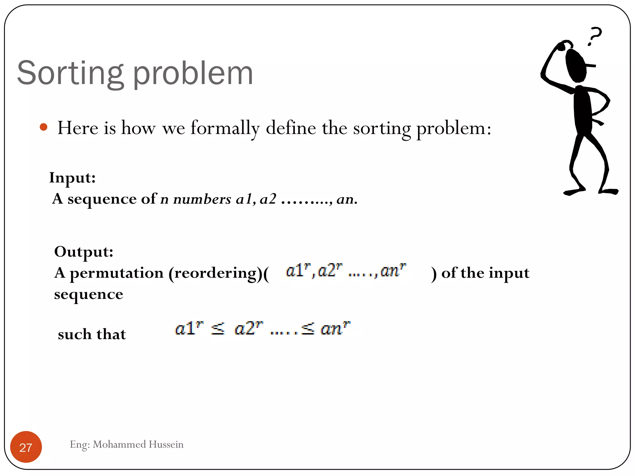
Prove 1 + 2 + 3 + … + n = n(n+1) / 2
Basis:
If n = 0, then 0 = 0(0+1) / 2
Inductive hypothesis:
Assume 1 + 2 + 3 + … + n = n(n+1) / 2
Step (show true for n+1):
1 + 2 + … + n + n+1 = (1 + 2 + …+ n) + (n+1)
= n(n+1)/2 + n+1 = [n(n+1) + 2(n+1)]/2
= (n+1)(n+2)/2 = (n+1)(n+1 + 1) / 2
n ( n +1) / 29 Eng: Mohammed Hussein
9](https://image.slidesharecdn.com/lecture2-130513060202-phpapp01/85/Iteration-induction-and-recursion-9-320.jpg)


![Selection Sort Algorithm
Eng: Mohammed Hussein28
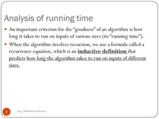
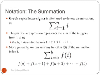
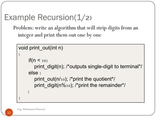
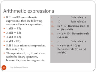
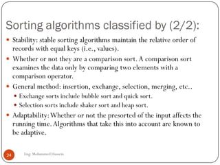
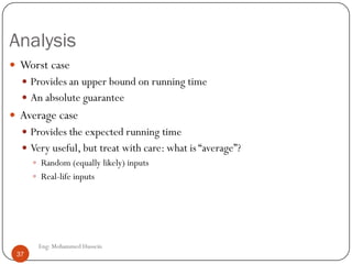
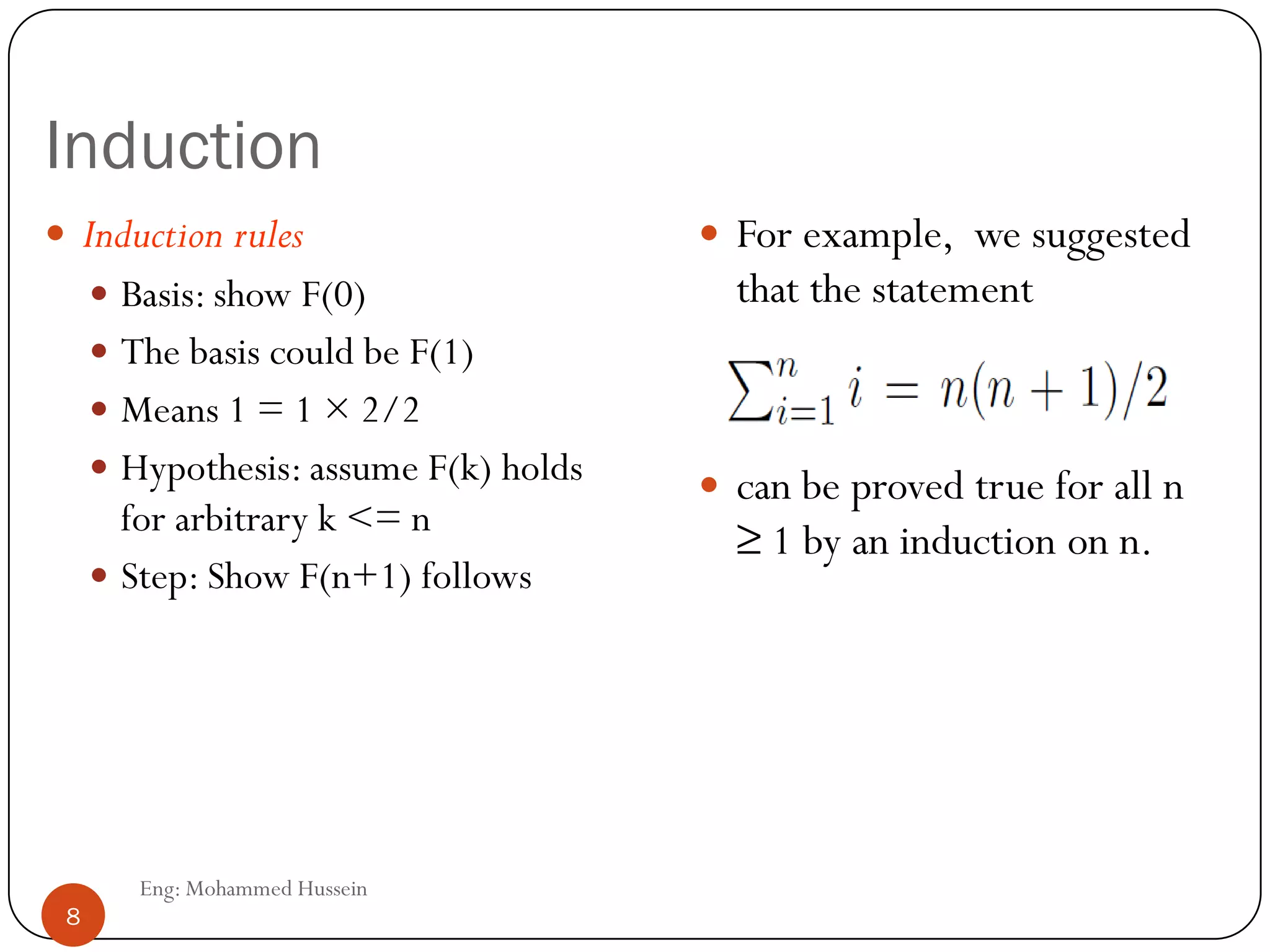
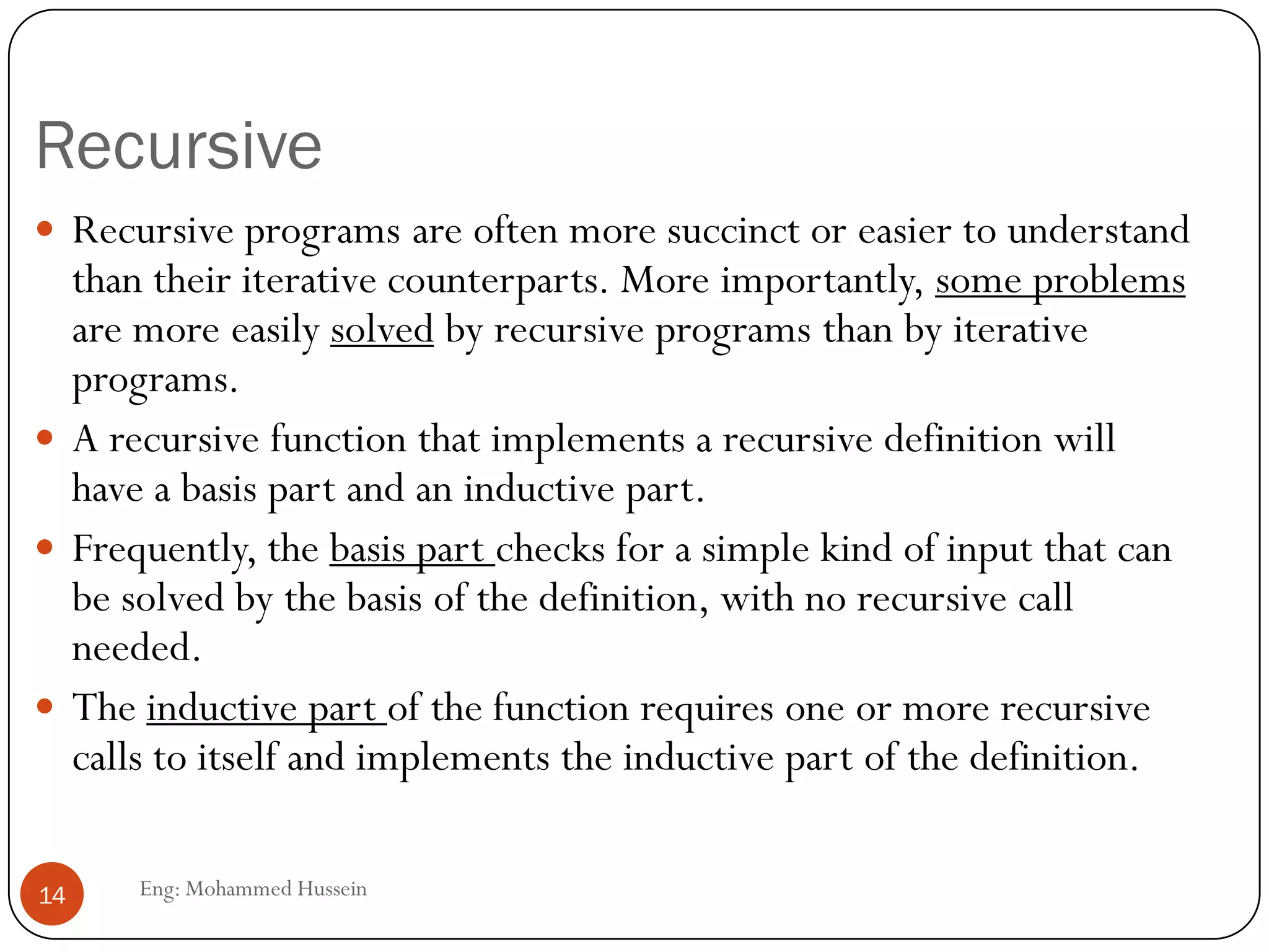
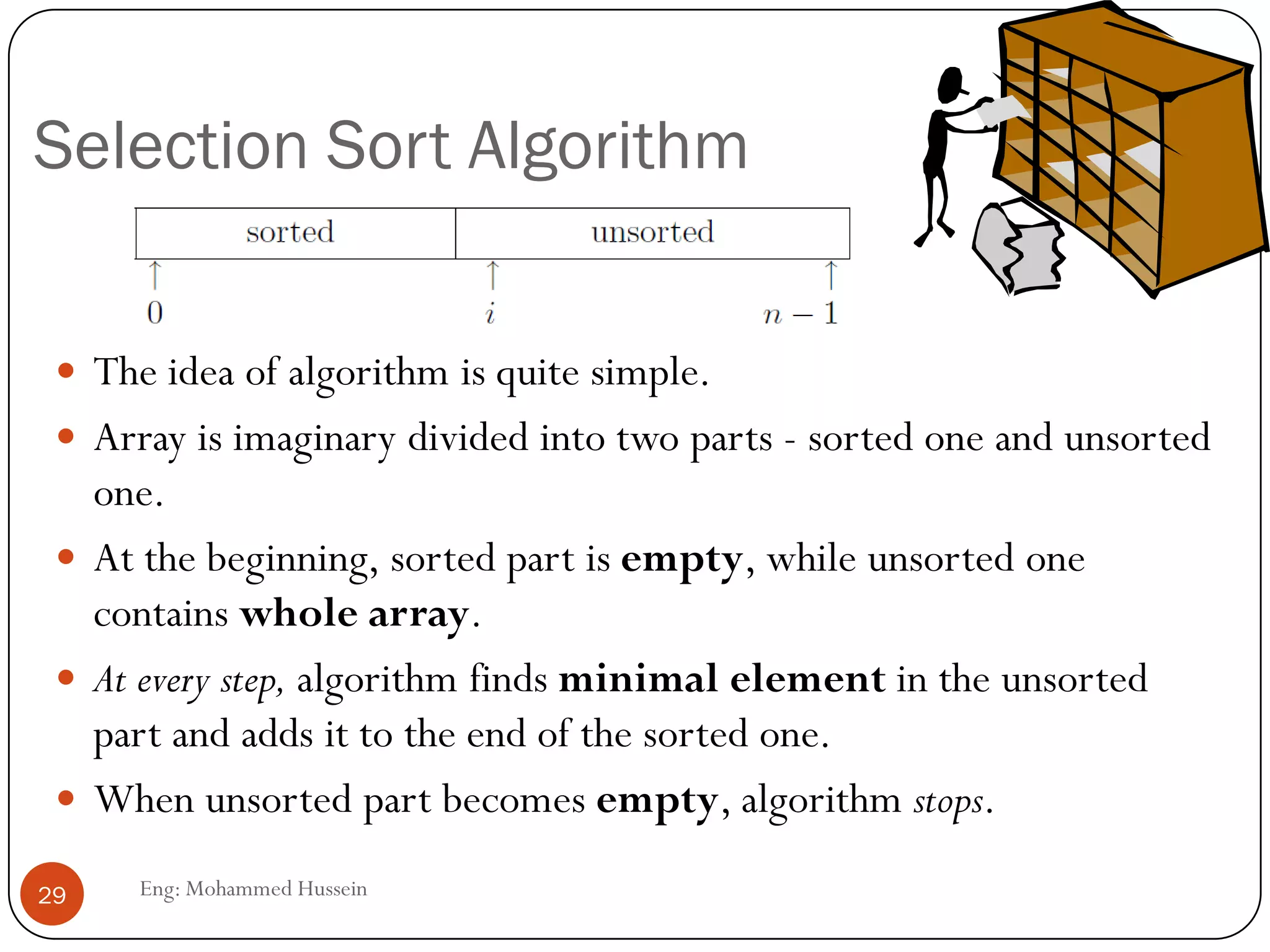
Suppose we have an array A of n integers that we wish to sort into
nondecreasing order.
We may do so by iterating a step in which a smallest element not yet part
of the sorted portion of the array is found and exchanged with the
element in the first position of the unsorted part of the array.
In the first iteration, we find (“select”) a smallest element among the
values found in the full arrayA[0..n-1] and exchange it withA[0].
In the second iteration, we find a smallest element in A[1..n-1] and
exchange it with A[1].
We continue these iterations.At the start of the i + 1st iteration,A[0..i-1]
contains the i smallest elements inA sorted in nondecreasing order, and
the remaining elements of the array are in no particular order.](https://image.slidesharecdn.com/lecture2-130513060202-phpapp01/85/Iteration-induction-and-recursion-28-320.jpg)

![Selection Sort Algorithm
Eng: Mohammed Hussein30
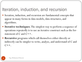
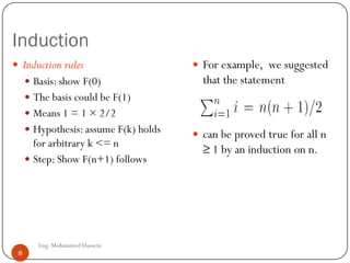
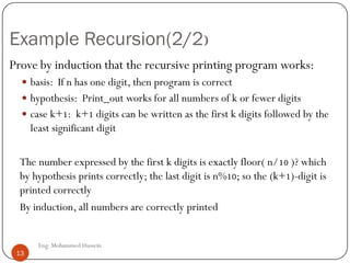
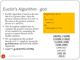
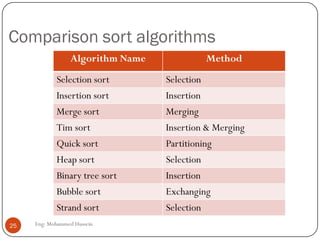
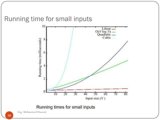
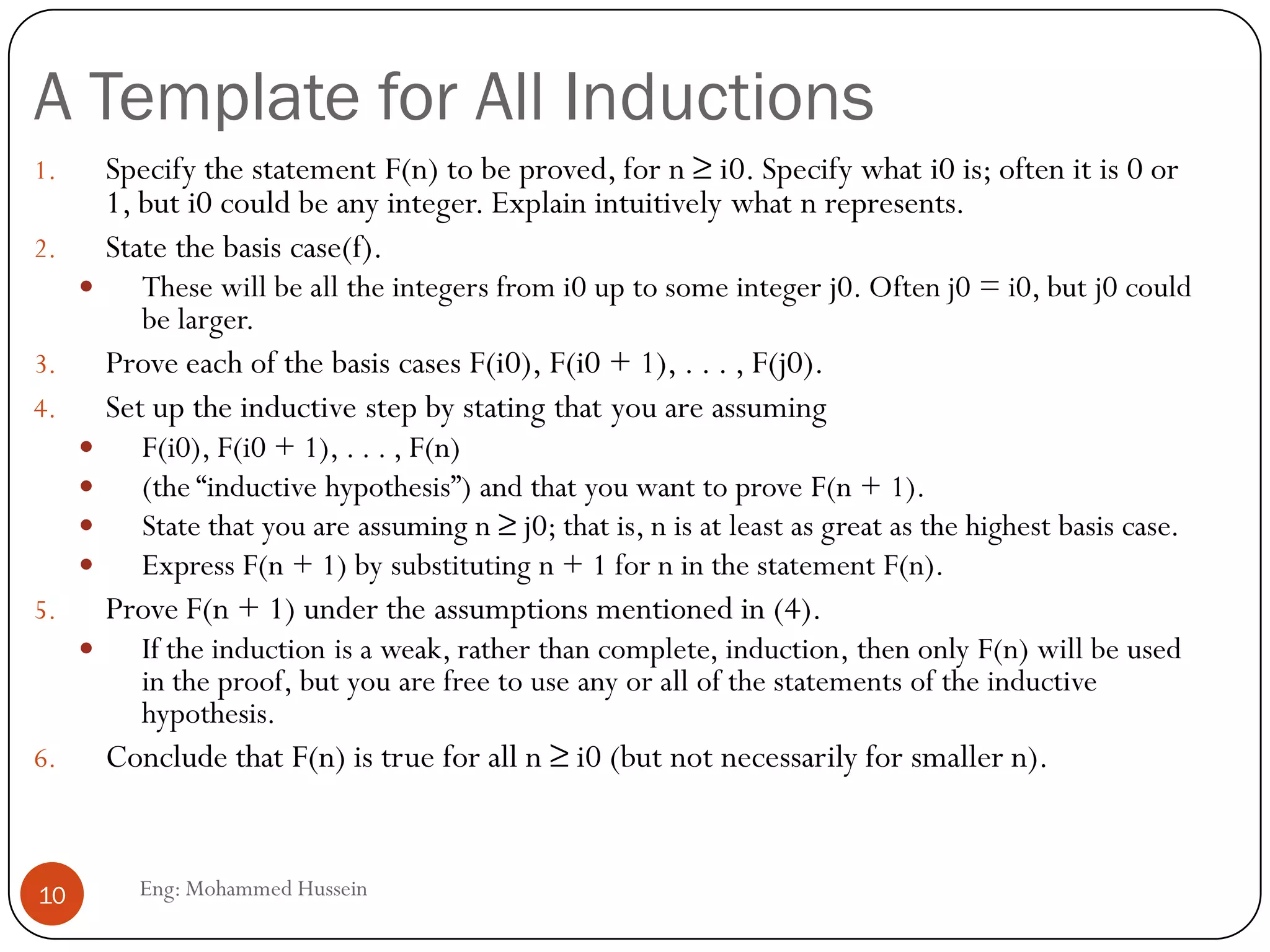
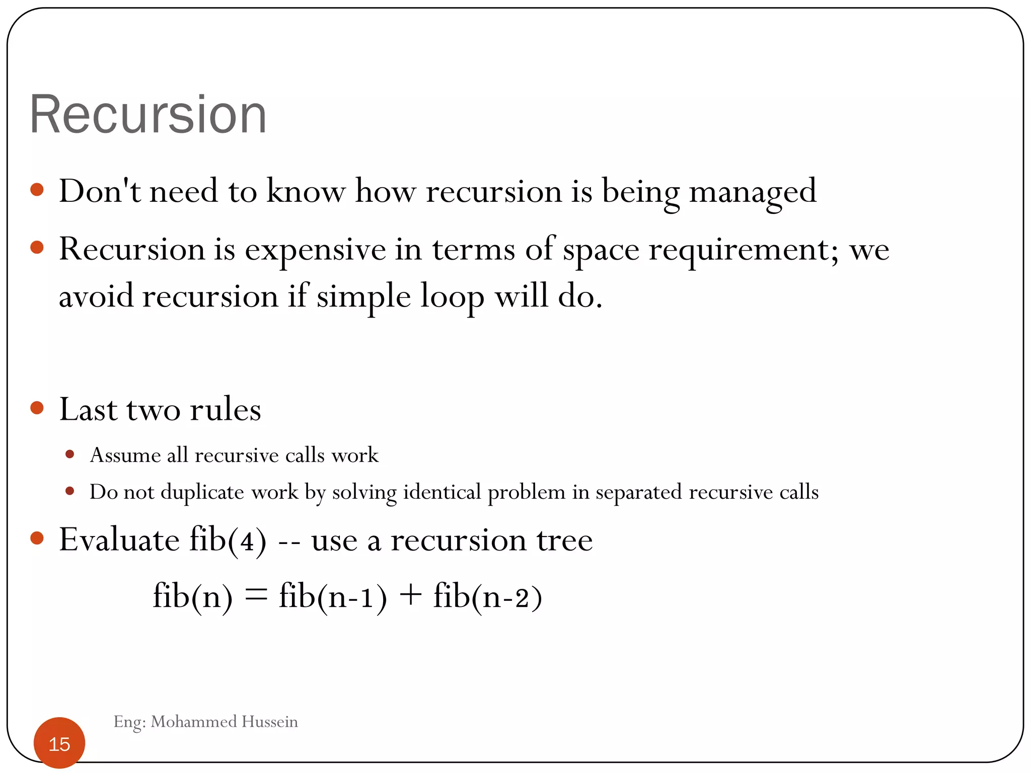
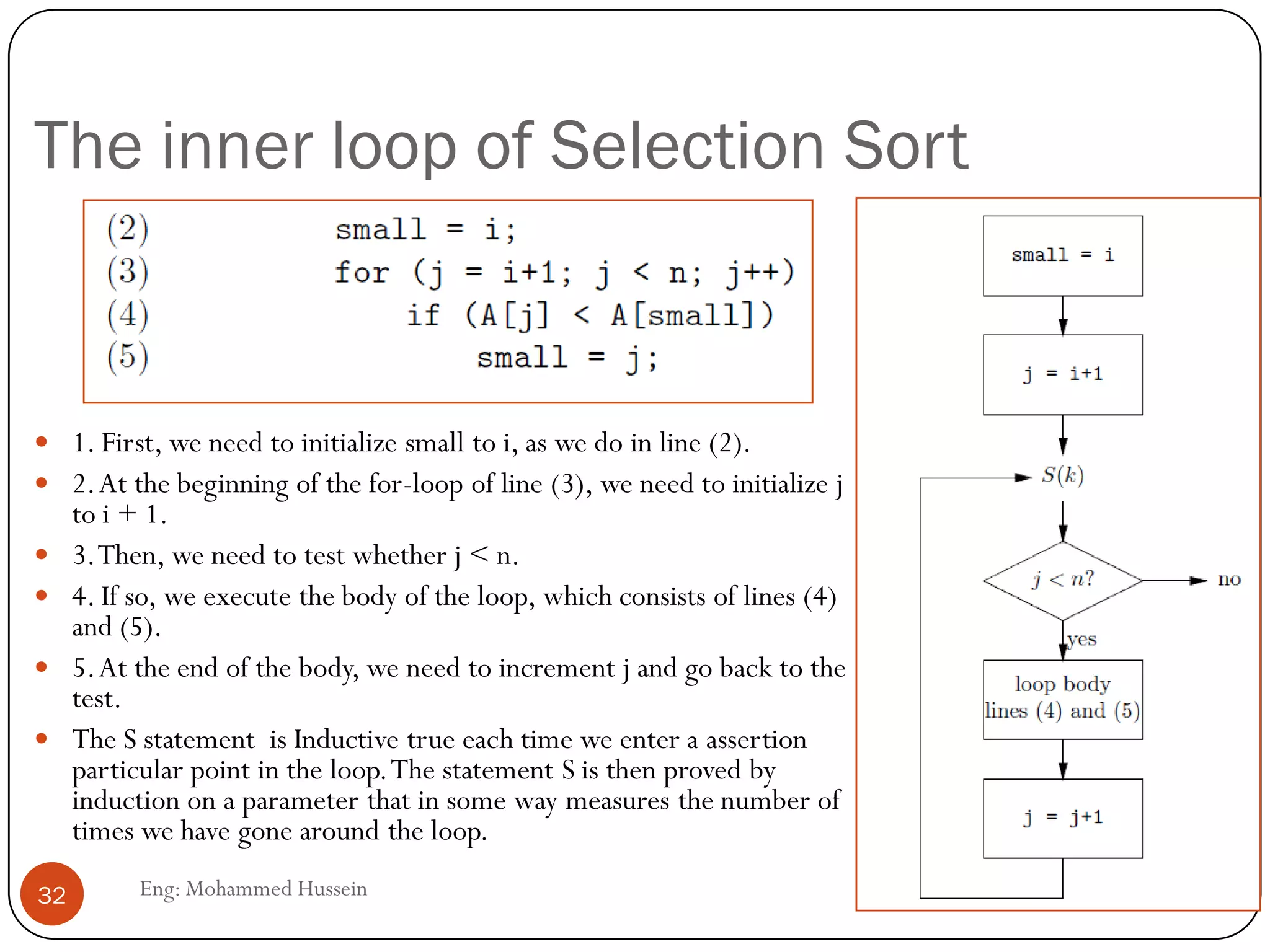
Lines (2) through (5) select a smallest element in the
unsorted part of the array, A[i..n-1]. We begin by
setting the small to i in line (2).
we set small to the index of the smallest element in
A[i..n-1] via for-loop of lines (3) through (5).And
small is set to j if A[j] has a smaller value than any of
the array elements in the range A[i..j-1].
In lines (6) to (8), we exchange the element in that
position with the element in A[i].
Notice that in order to swap two elements, we need a
temporary place to store one of them.Thus, we move
the value in A[small] to temp at line (6), move the
value in A[i] to A[small] at line (7), and finally move
the value originally in A[small] from temp to A[i] at
line (8).](https://image.slidesharecdn.com/lecture2-130513060202-phpapp01/85/Iteration-induction-and-recursion-30-320.jpg)
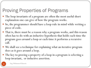
![The inner loop of Selection Sort
Eng: Mohammed Hussein33
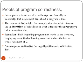
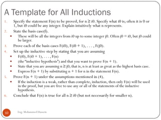
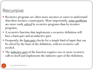
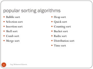
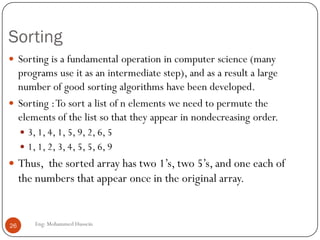
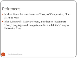
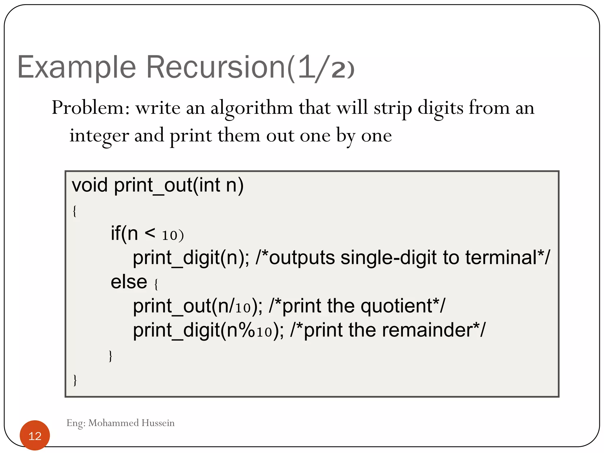
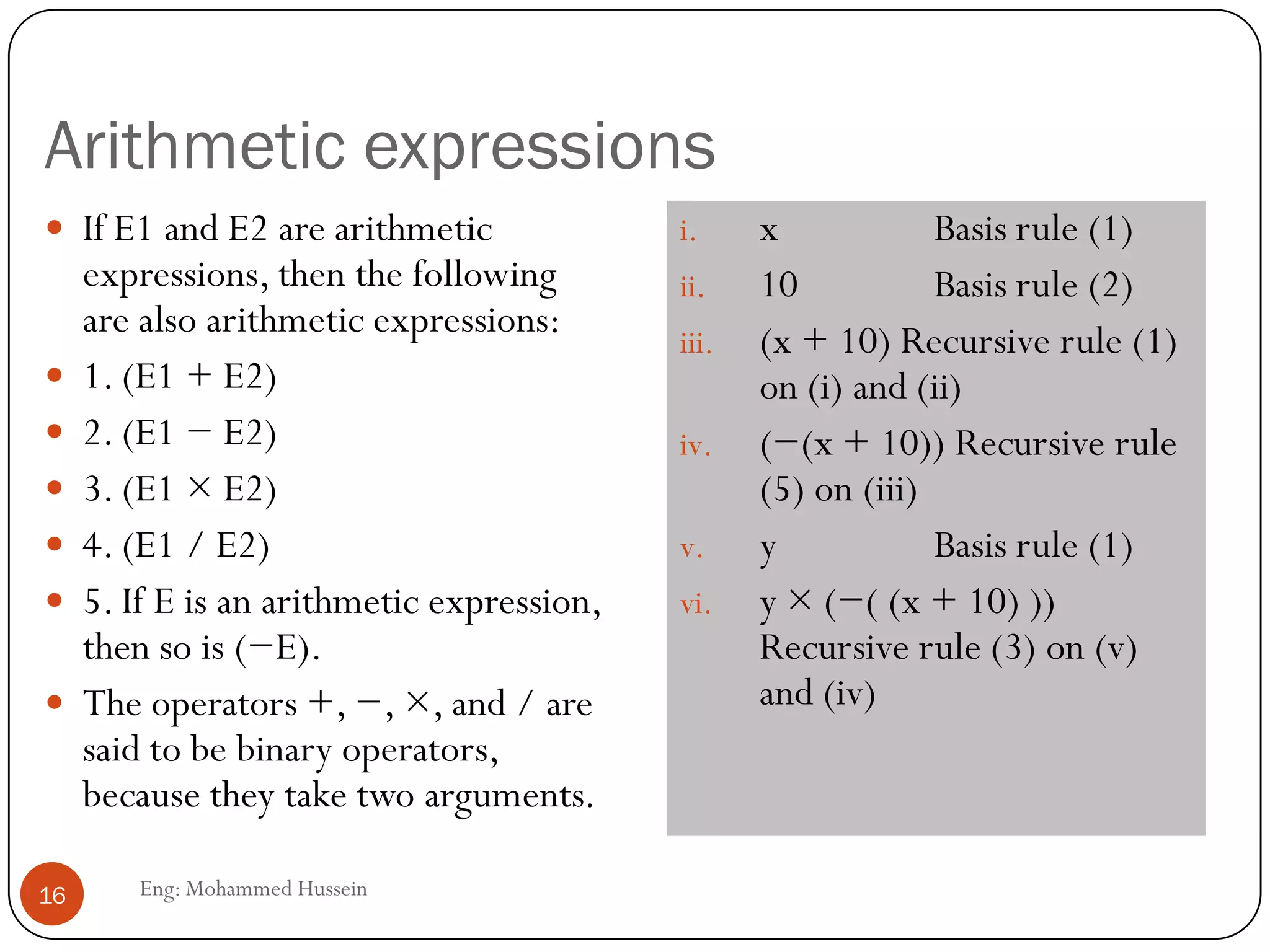
we see a point just before the test that is labeled by a
loop-invariant statement we have called S(k);
The first time we reach the test, j has the value i + 1
and small has the value i.
The second time we reach the test, j has the value i+2,
because j has been incremented once.
Because the body (lines 4 and 5) sets small to i + 1 if
A[i + 1] is less thanA[i], we see that small is the index
of whichever of A[i] andA[i + 1] is smaller
Similarly, the third time we reach the test, the value of j
is i + 3 and small is the index of the smallest of
A[i..i+2].
S(k): If we reach the test for j < n in the for-statement
of line (3) with k as the value of loop index j, then the
value of small is the index of the smallest of A[i..k-1].](https://image.slidesharecdn.com/lecture2-130513060202-phpapp01/85/Iteration-induction-and-recursion-33-320.jpg)


![Induction Example:
Gaussian Closed Form
Prove 1 + 2 + 3 + … + n = n(n+1) / 2
Basis:
If n = 0, then 0 = 0(0+1) / 2
Inductive hypothesis:
Assume 1 + 2 + 3 + … + n = n(n+1) / 2
Step (show true for n+1):
1 + 2 + … + n + n+1 = (1 + 2 + …+ n) + (n+1)
= n(n+1)/2 + n+1 = [n(n+1) + 2(n+1)]/2
= (n+1)(n+2)/2 = (n+1)(n+1 + 1) / 2
n ( n +1) / 29 Eng: Mohammed Hussein
9](https://image.slidesharecdn.com/lecture2-130513060202-phpapp01/75/Iteration-induction-and-recursion-9-2048.jpg)


![Selection Sort Algorithm
Eng: Mohammed Hussein28
Suppose we have an array A of n integers that we wish to sort into
nondecreasing order.
We may do so by iterating a step in which a smallest element not yet part
of the sorted portion of the array is found and exchanged with the
element in the first position of the unsorted part of the array.
In the first iteration, we find (“select”) a smallest element among the
values found in the full arrayA[0..n-1] and exchange it withA[0].
In the second iteration, we find a smallest element in A[1..n-1] and
exchange it with A[1].
We continue these iterations.At the start of the i + 1st iteration,A[0..i-1]
contains the i smallest elements inA sorted in nondecreasing order, and
the remaining elements of the array are in no particular order.](https://image.slidesharecdn.com/lecture2-130513060202-phpapp01/75/Iteration-induction-and-recursion-28-2048.jpg)
![Selection Sort Algorithm
Eng: Mohammed Hussein30
Lines (2) through (5) select a smallest element in the
unsorted part of the array, A[i..n-1]. We begin by
setting the small to i in line (2).
we set small to the index of the smallest element in
A[i..n-1] via for-loop of lines (3) through (5).And
small is set to j if A[j] has a smaller value than any of
the array elements in the range A[i..j-1].
In lines (6) to (8), we exchange the element in that
position with the element in A[i].
Notice that in order to swap two elements, we need a
temporary place to store one of them.Thus, we move
the value in A[small] to temp at line (6), move the
value in A[i] to A[small] at line (7), and finally move
the value originally in A[small] from temp to A[i] at
line (8).](https://image.slidesharecdn.com/lecture2-130513060202-phpapp01/75/Iteration-induction-and-recursion-30-2048.jpg)
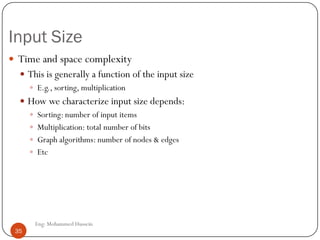
![The inner loop of Selection Sort
Eng: Mohammed Hussein33
we see a point just before the test that is labeled by a
loop-invariant statement we have called S(k);
The first time we reach the test, j has the value i + 1
and small has the value i.
The second time we reach the test, j has the value i+2,
because j has been incremented once.
Because the body (lines 4 and 5) sets small to i + 1 if
A[i + 1] is less thanA[i], we see that small is the index
of whichever of A[i] andA[i + 1] is smaller
Similarly, the third time we reach the test, the value of j
is i + 3 and small is the index of the smallest of
A[i..i+2].
S(k): If we reach the test for j < n in the for-statement
of line (3) with k as the value of loop index j, then the
value of small is the index of the smallest of A[i..k-1].](https://image.slidesharecdn.com/lecture2-130513060202-phpapp01/75/Iteration-induction-and-recursion-33-2048.jpg)

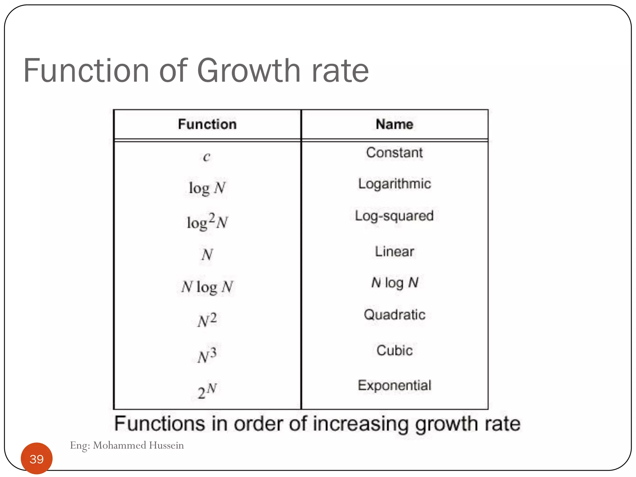

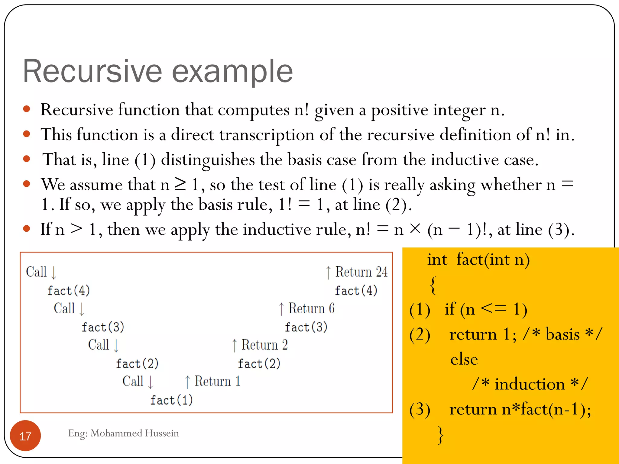
The document discusses various topics related to analyzing algorithms, including: i. Analysis of running time and using recurrence equations to predict how long recursive algorithms take on different input sizes. ii. Iteration, induction, and recursion as fundamental concepts in data structures and algorithms. Recursive programs can sometimes be simpler than iterative programs. iii. Proving properties of programs formally or informally, such as proving statements are true for each iteration of a loop or recursive call of a function. This is often done using induction.


