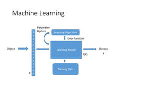
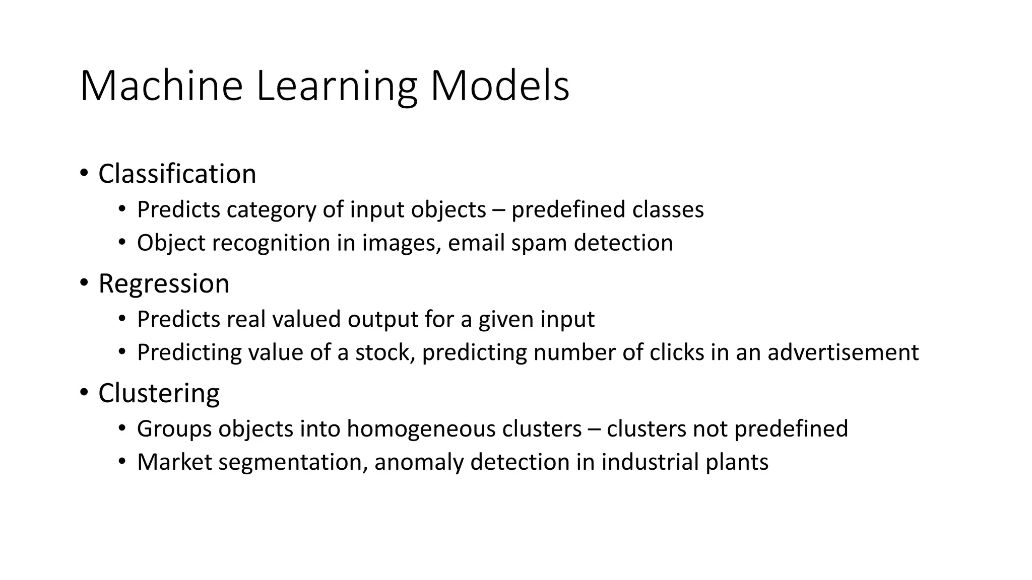
Machine Learning Algorithms Introduction.pdf

Introduction to Machine
Learning Algorithms
Pabitra Mitra
Indian Institute of Technology Kharagpur
pabitra@cse.iitkgp.ac.in

Machine Learning
• Learning Algorithms/Systems: Performance improvement with
experience, generalize to unseen input
• Example:
• Face recognition
• Email spam detection
• Market segmentation
• Rainfall forecasting
• Inductive inference – Data to Model

Machine Learning
R
e
p
r
e
s
e
n
t
a
t
i
o
n
Object Learning Model
Training Data
Learning Algorithm
Error function
Parameter
Update
Output
X
y
f(X)

Machine Learning Models
• Classification
• Predicts category of input objects – predefined classes
• Object recognition in images, email spam detection
• Regression
• Predicts real valued output for a given input
• Predicting value of a stock, predicting number of clicks in an advertisement
• Clustering
• Groups objects into homogeneous clusters – clusters not predefined
• Market segmentation, anomaly detection in industrial plants

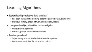
Learning Algorithms
• Supervised (predictive data analysis)
• For each input in the training data the desired output is known
• Previous history, ground truth, annotations, labels
• Unsupervised (explorative data analysis)
• Output is not specified
• Natural groups are to be determined
• Semi-supervised
• Supervisory output available for few data points
• Output not available for most data points

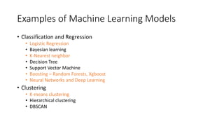
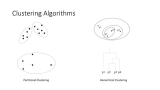
Examples of Machine Learning Models
• Classification and Regression
• Logistic Regression
• Bayesian learning
• K-Nearest neighbor
• Decision Tree
• Support Vector Machine
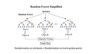
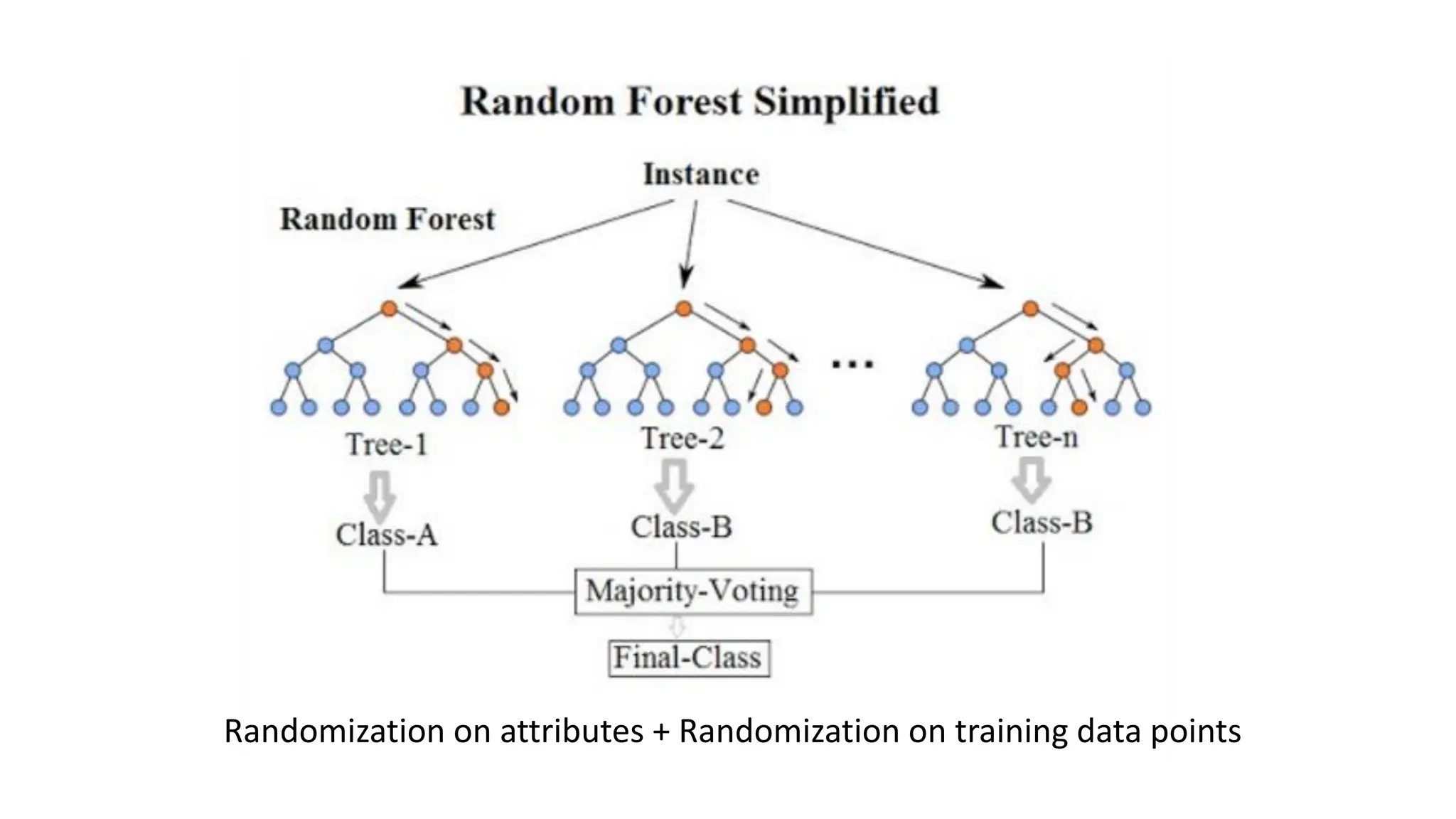
• Boosting – Random Forests, Xgboost
• Neural Networks and Deep Learning
• Clustering
• K-means clustering
• Hierarchical clustering
• DBSCAN

Linear Regression
X
y
Prediction Model: y = 𝑓 𝑋, 𝛽 + ε
𝑓 𝑋, 𝛽 = 𝛽0 + 𝛽1𝑋 + ε
Linear Regression: Find 𝛽 that minimises the sum squared error

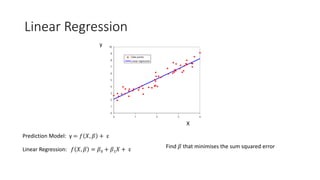
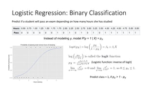
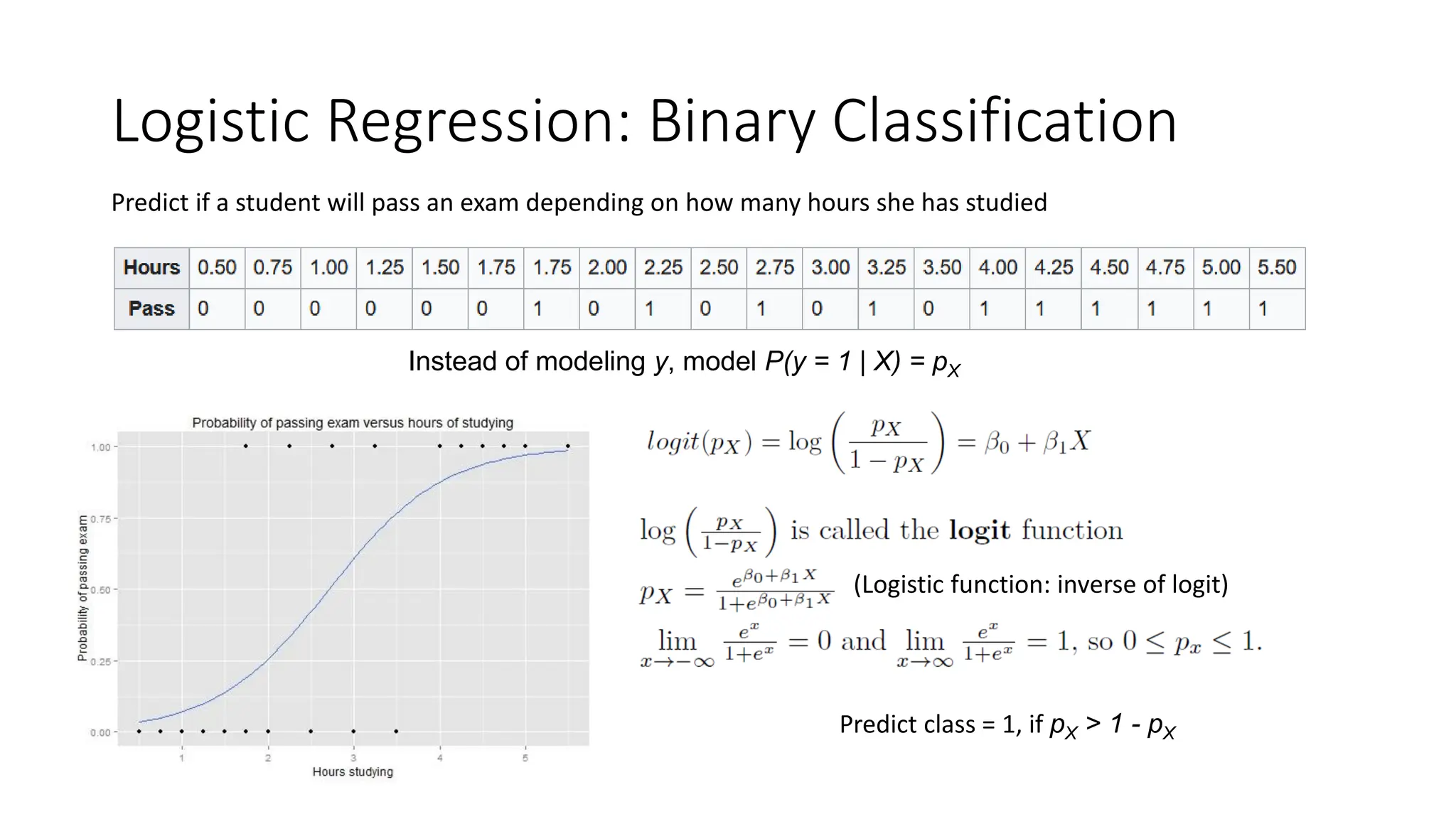
Logistic Regression: Binary Classification
Predict if a student will pass an exam depending on how many hours she has studied
Instead of modeling y, model P(y = 1 | X) = pX
(Logistic function: inverse of logit)
Predict class = 1, if pX > 1 - pX

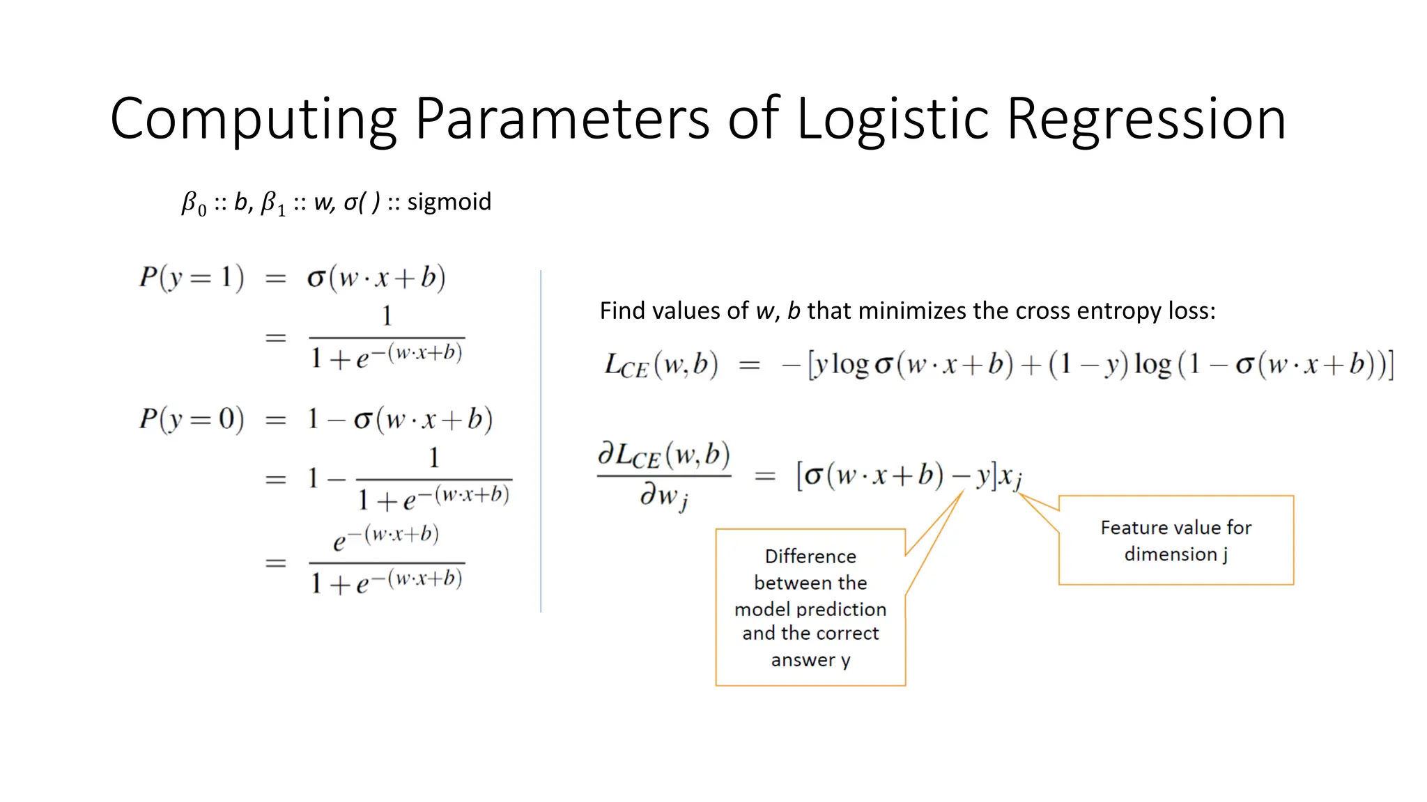
Computing Parameters of Logistic Regression
𝛽0 :: b, 𝛽1 :: w, σ( ) :: sigmoid
Find values of w, b that minimizes the cross entropy loss:

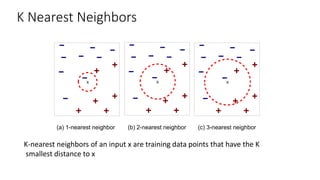
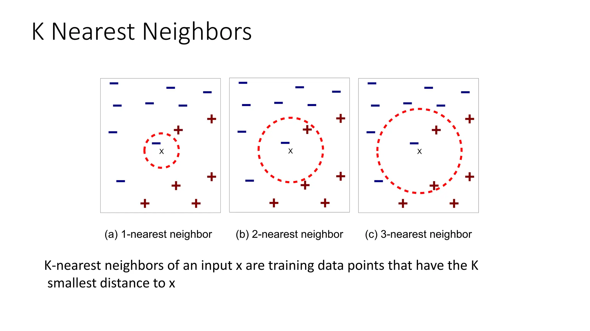
K Nearest Neighbors
X X X
(a) 1-nearest neighbor (b) 2-nearest neighbor (c) 3-nearest neighbor
K-nearest neighbors of an input x are training data points that have the K
smallest distance to x

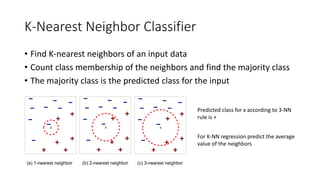
K-Nearest Neighbor Classifier
• Find K-nearest neighbors of an input data
• Count class membership of the neighbors and find the majority class
• The majority class is the predicted class for the input
X X X
(a) 1-nearest neighbor (b) 2-nearest neighbor (c) 3-nearest neighbor
Predicted class for x according to 3-NN
rule is +
For K-NN regression predict the average
value of the neighbors

Nearest-Neighbor Classifiers: Design Choices
– The value of k, the number of nearest neighbors to retrieve
– Distance Metric to compute distance between data points

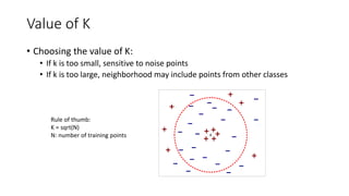
Value of K
• Choosing the value of K:
• If k is too small, sensitive to noise points
• If k is too large, neighborhood may include points from other classes
X
Rule of thumb:
K = sqrt(N)
N: number of training points

Distance Measure: Scale Effects
• Different features may have different measurement scales
• E.g., patient weight in kg (range [50,200]) vs. blood protein values in ng/L ([-3,3])
• Consequences
• Patient weight will have a greater influence on the distance between samples
• May bias the performance of the classifier
• Transform raw feature values into z-scores
• is the value for the ith sample and jth feature
• is the average of all inputs or feature j
• is the standard deviation of all inputs over all input samples
• Range and scale of z-scores should be similar (providing distributions of raw feature values are alike)
zij =
xij - mj
s j
xij
mj
s j

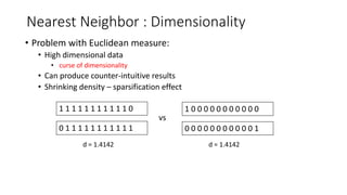
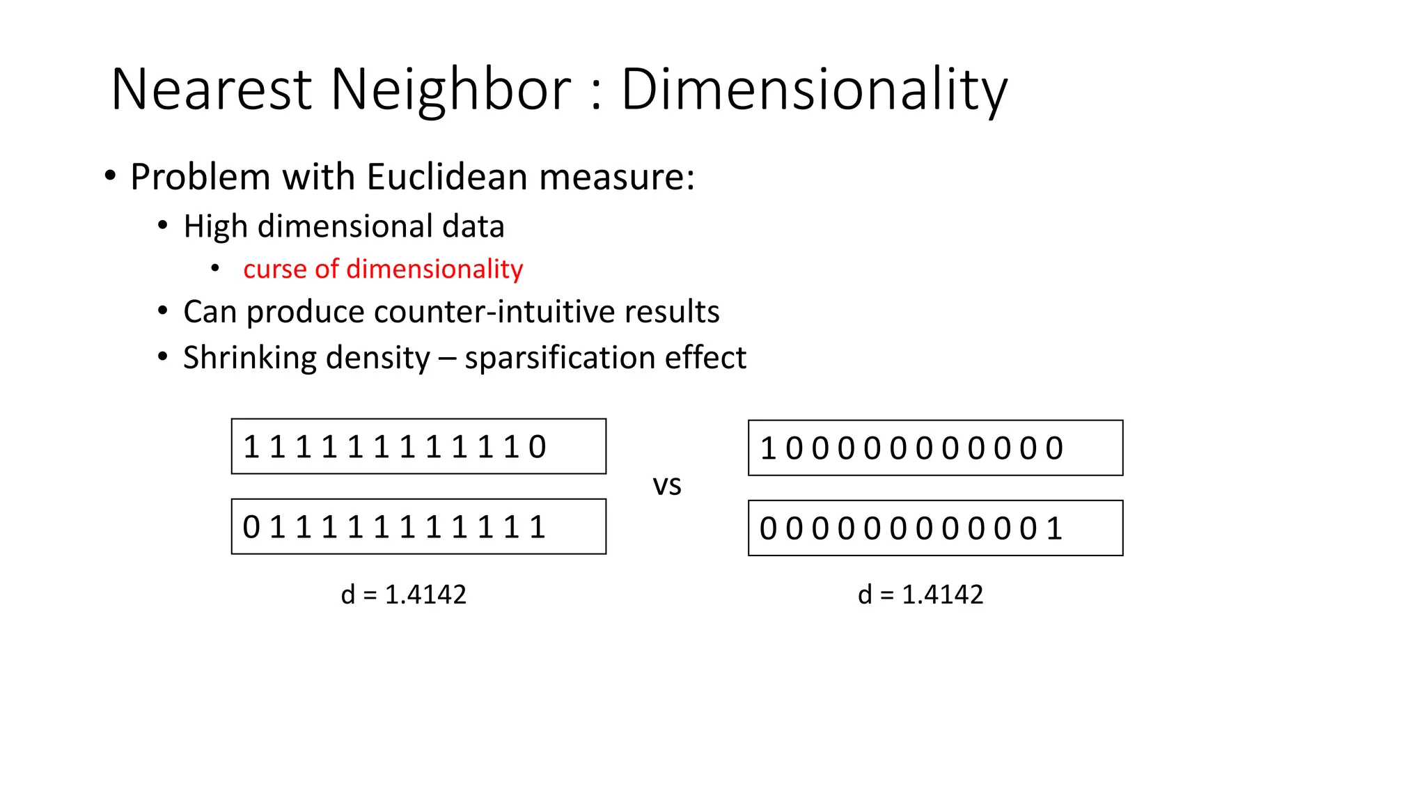
Nearest Neighbor : Dimensionality
• Problem with Euclidean measure:
• High dimensional data
• curse of dimensionality
• Can produce counter-intuitive results
• Shrinking density – sparsification effect
1 1 1 1 1 1 1 1 1 1 1 0
0 1 1 1 1 1 1 1 1 1 1 1
1 0 0 0 0 0 0 0 0 0 0 0
0 0 0 0 0 0 0 0 0 0 0 1
vs
d = 1.4142 d = 1.4142

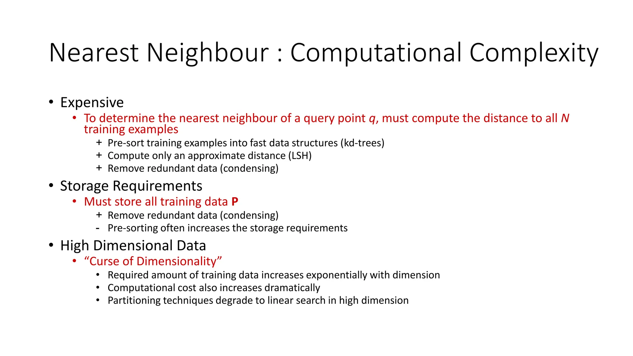
Nearest Neighbour : Computational Complexity
• Expensive
• To determine the nearest neighbour of a query point q, must compute the distance to all N
training examples
+ Pre-sort training examples into fast data structures (kd-trees)
+ Compute only an approximate distance (LSH)
+ Remove redundant data (condensing)
• Storage Requirements
• Must store all training data P
+ Remove redundant data (condensing)
- Pre-sorting often increases the storage requirements
• High Dimensional Data
• “Curse of Dimensionality”
• Required amount of training data increases exponentially with dimension
• Computational cost also increases dramatically
• Partitioning techniques degrade to linear search in high dimension

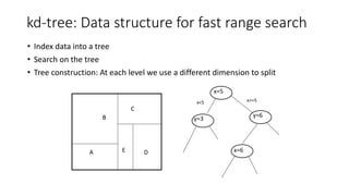
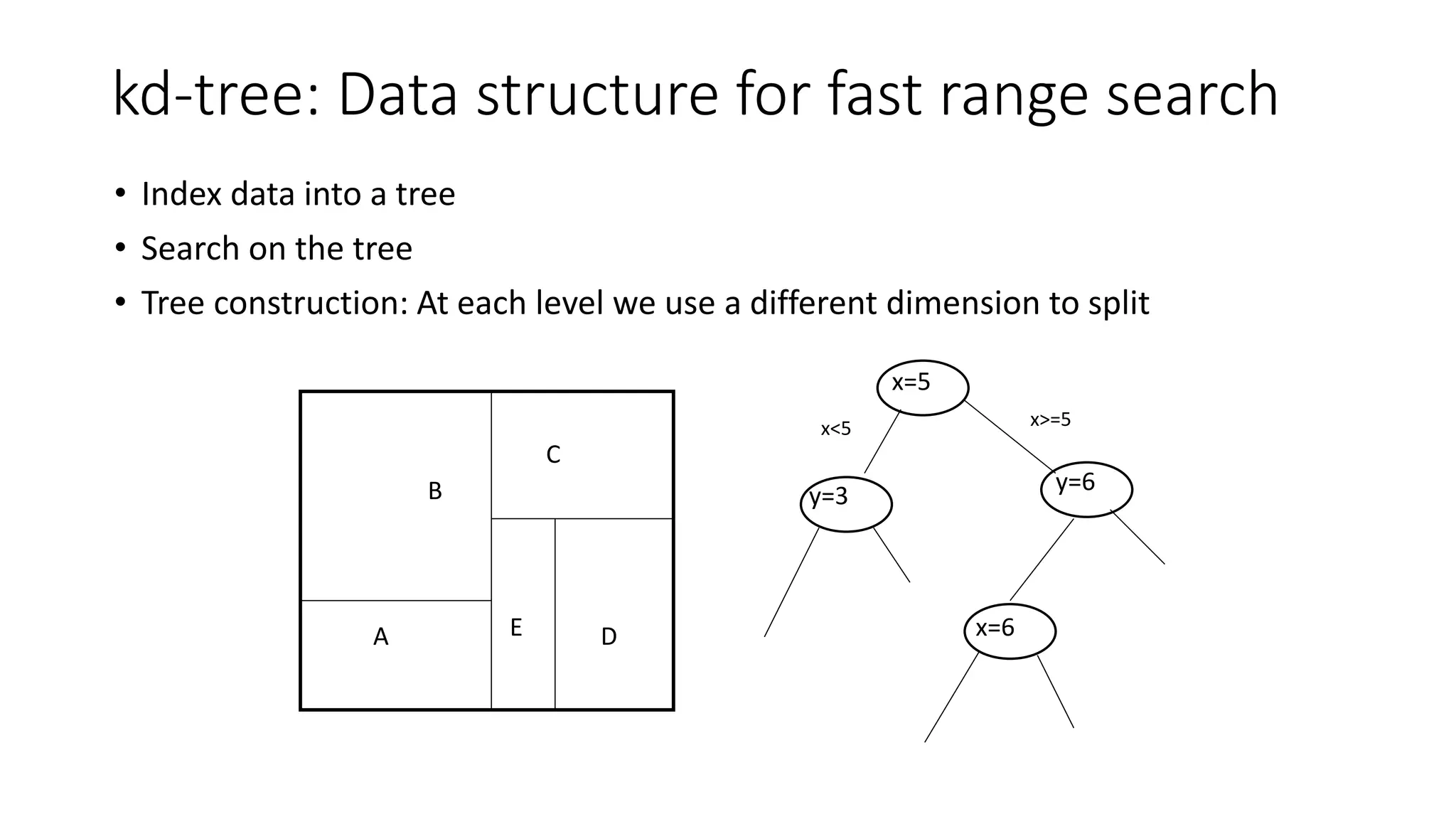
kd-tree: Data structure for fast range search
• Index data into a tree
• Search on the tree
• Tree construction: At each level we use a different dimension to split
x=5
y=3
y=6
x=6
A
B
C
D
E
x<5 x>=5

Ensemble Classifier
S Training
Data
S1 S2 Sn
Multiple Data
Sets
C1 C2 Cn
Multiple
Classifiers
H
Combined
Classifier

Bagging (Bootstrapped Aggregation)
Bootstrapping: Sampling with replacement from the original data set

Decision Trees
Leaves denote class decisions, other nodes denote attributes of data points

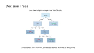
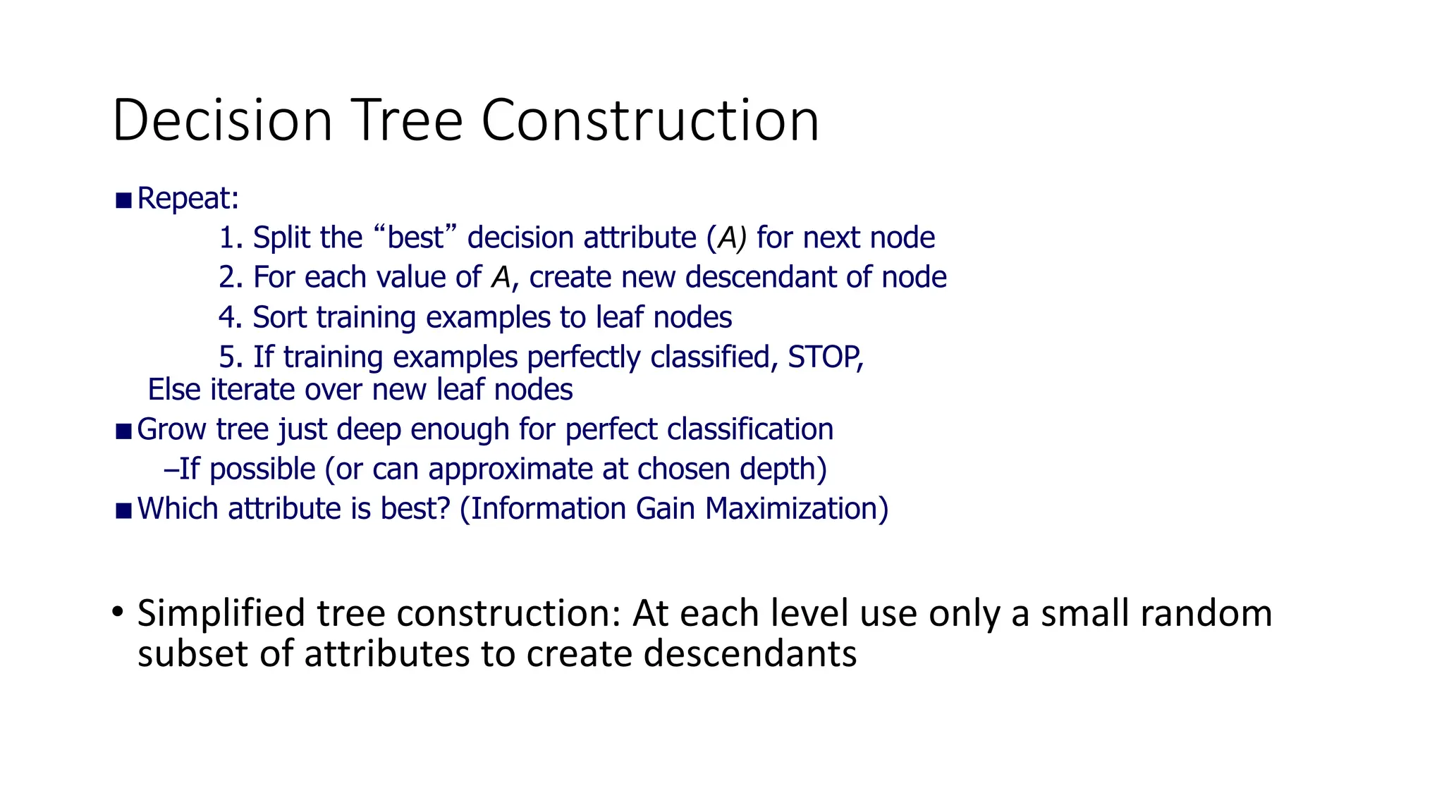
Decision Tree Construction
Repeat:
1. Split the “best” decision attribute (A) for next node
2. For each value of A, create new descendant of node
4. Sort training examples to leaf nodes
5. If training examples perfectly classified, STOP,
Else iterate over new leaf nodes
Grow tree just deep enough for perfect classification
–If possible (or can approximate at chosen depth)
Which attribute is best? (Information Gain Maximization)
• Simplified tree construction: At each level use only a small random
subset of attributes to create descendants

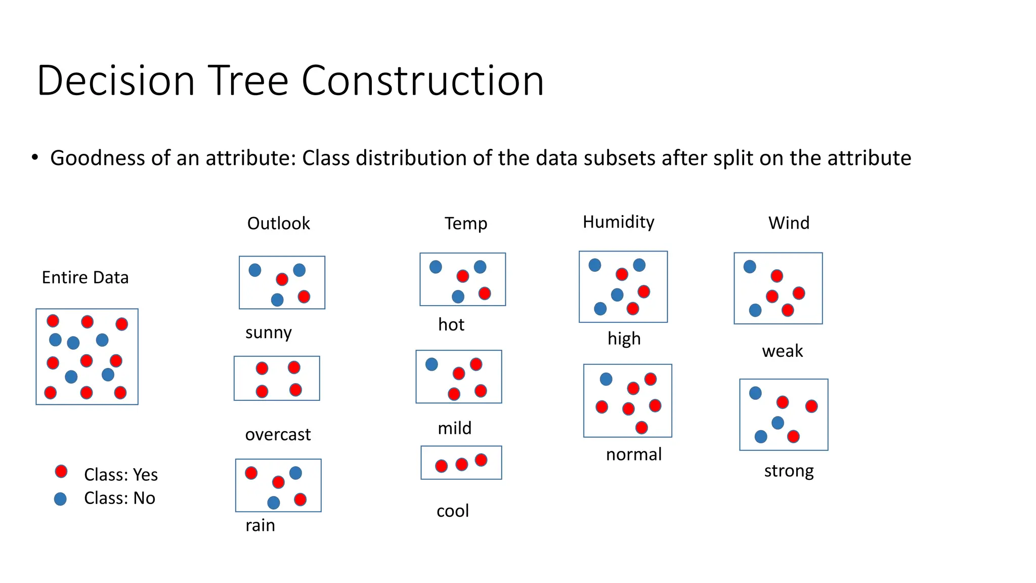
Decision Tree Construction
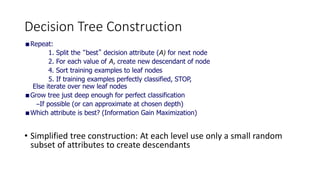
• Goodness of an attribute: Class distribution of the data subsets after split on the attribute
Class: Yes
Class: No
Entire Data
Outlook Temp Humidity Wind
sunny
overcast
rain
hot
mild
cool
high
normal
weak
strong

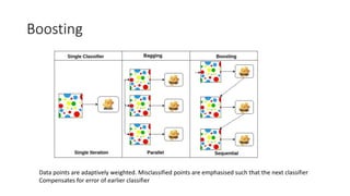
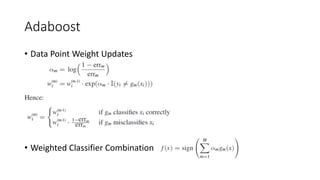
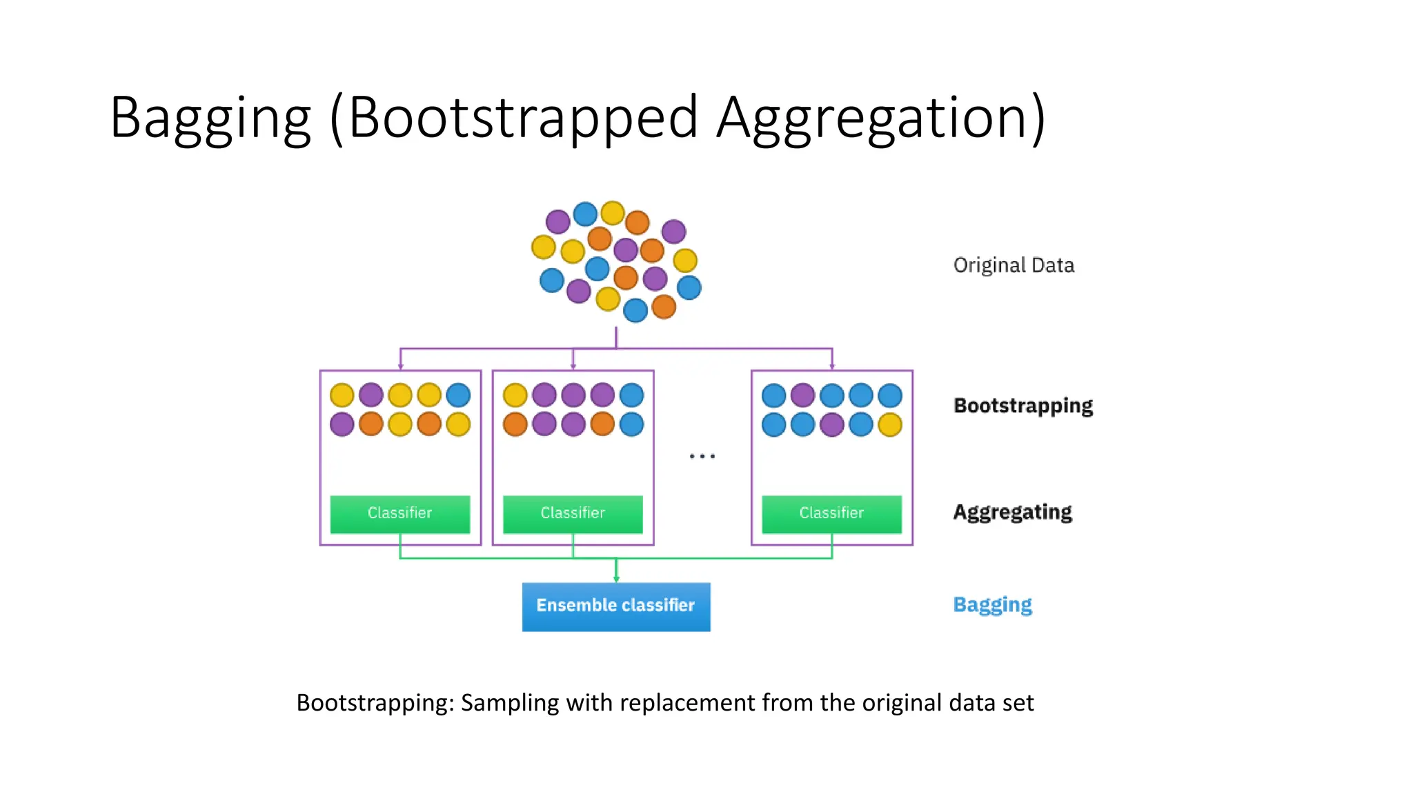
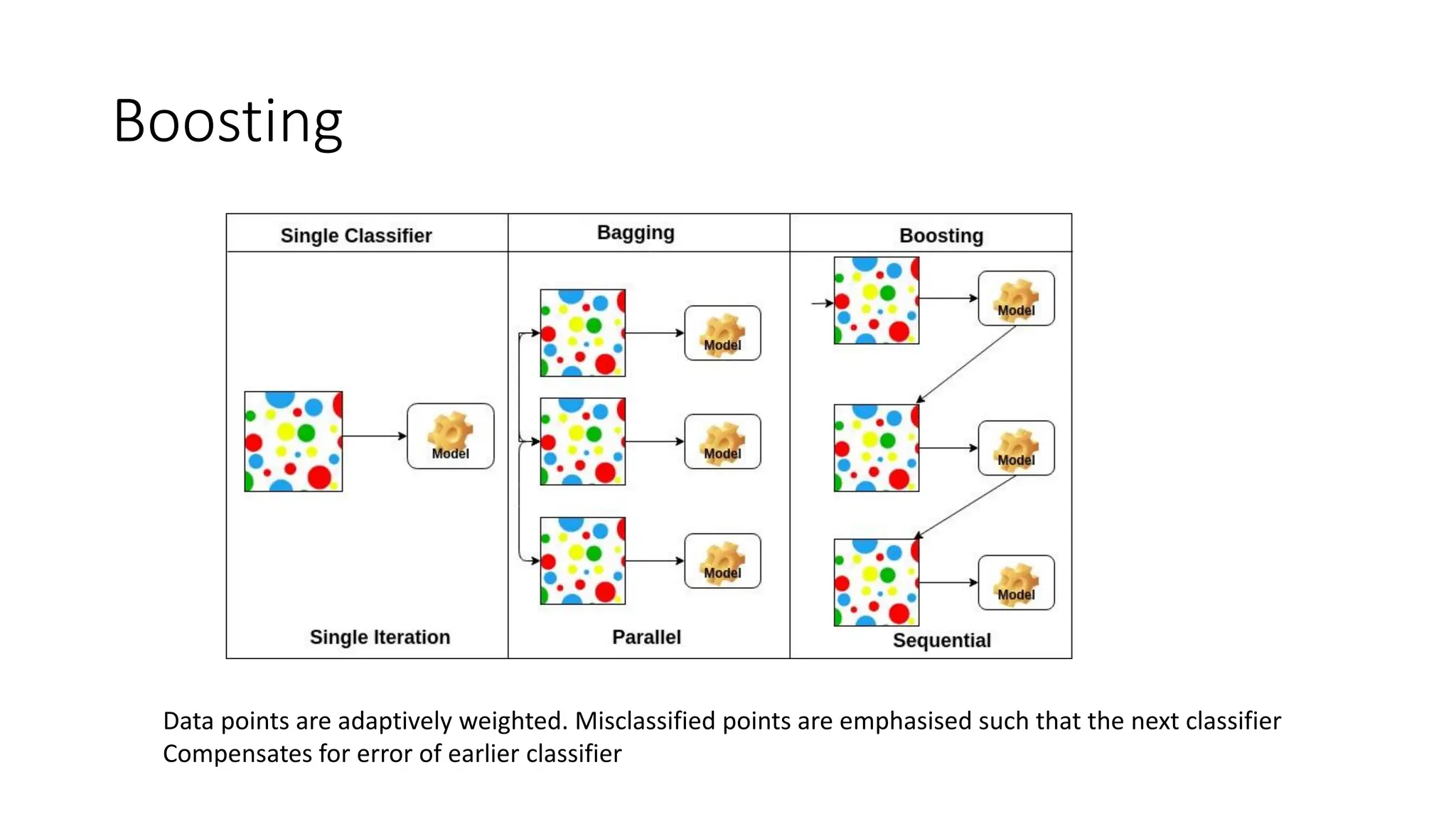
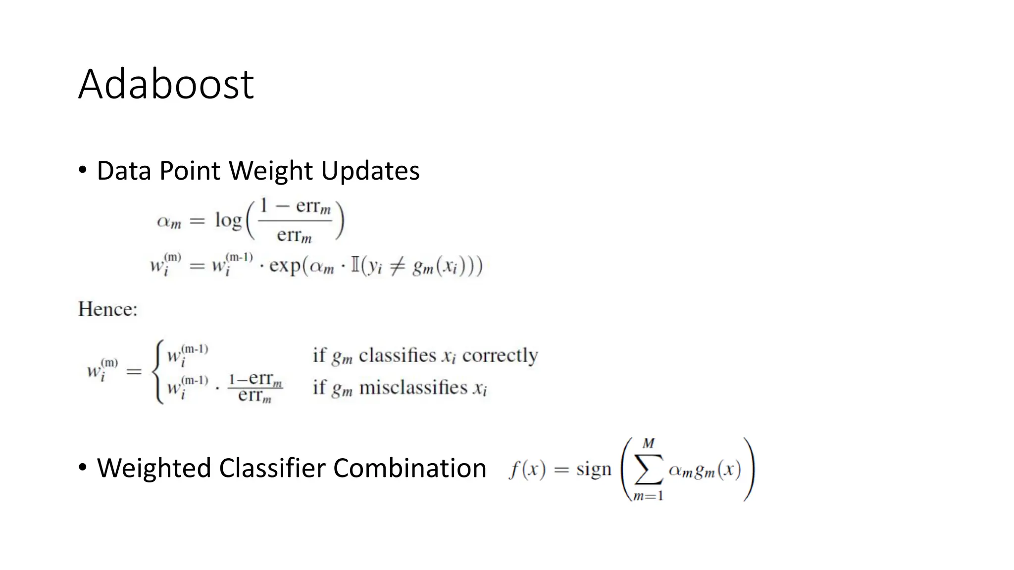
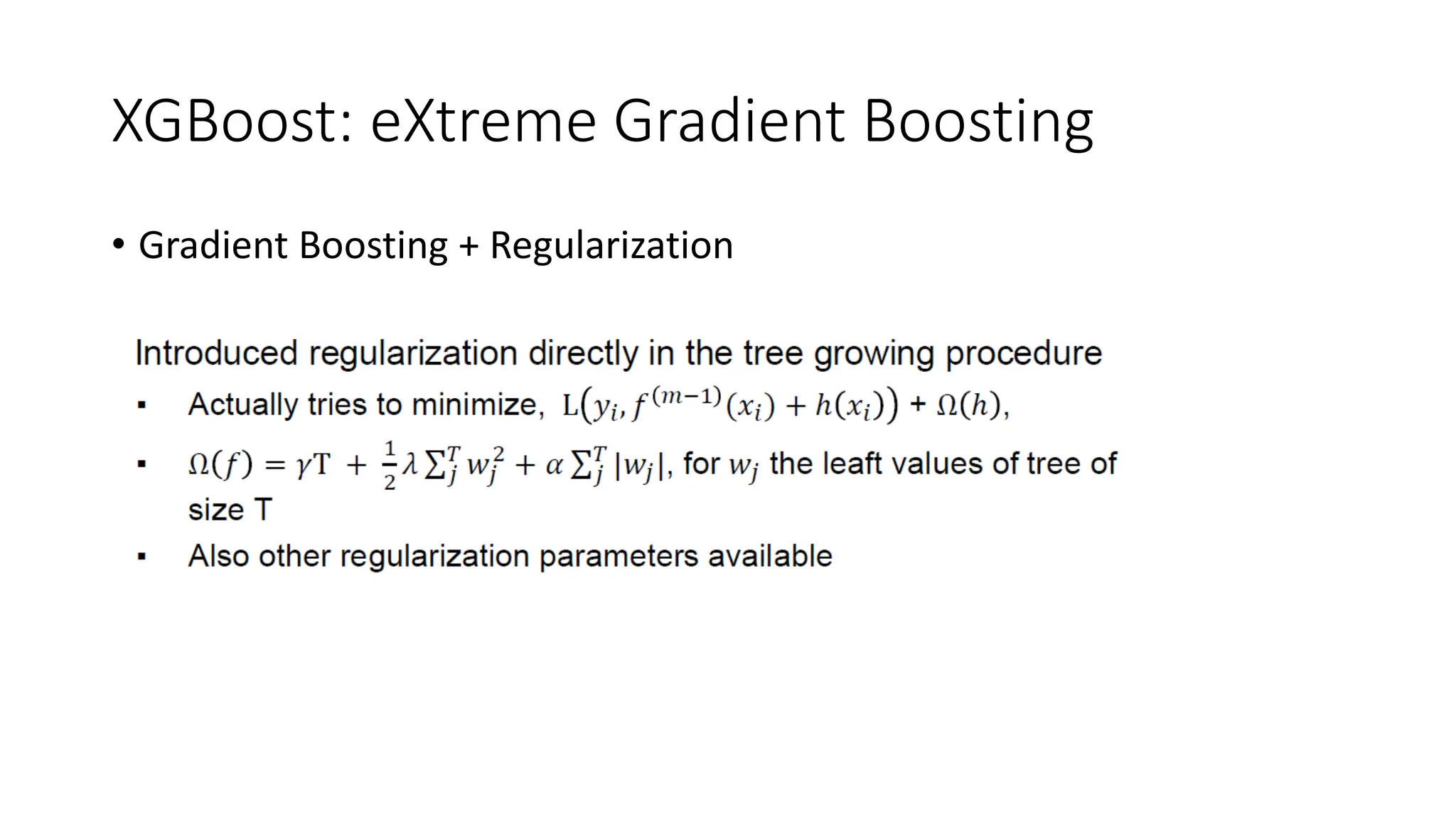
Randomization on attributes + Randomization on training data points

Boosting
Data points are adaptively weighted. Misclassified points are emphasised such that the next classifier
Compensates for error of earlier classifier

Adaboost
• Data Point Weight Updates
• Weighted Classifier Combination

Forward Stagewise Additive Modelling
Adaboost FSAM for exponential loss.

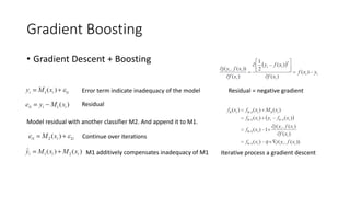
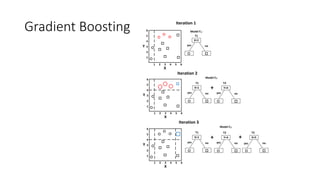
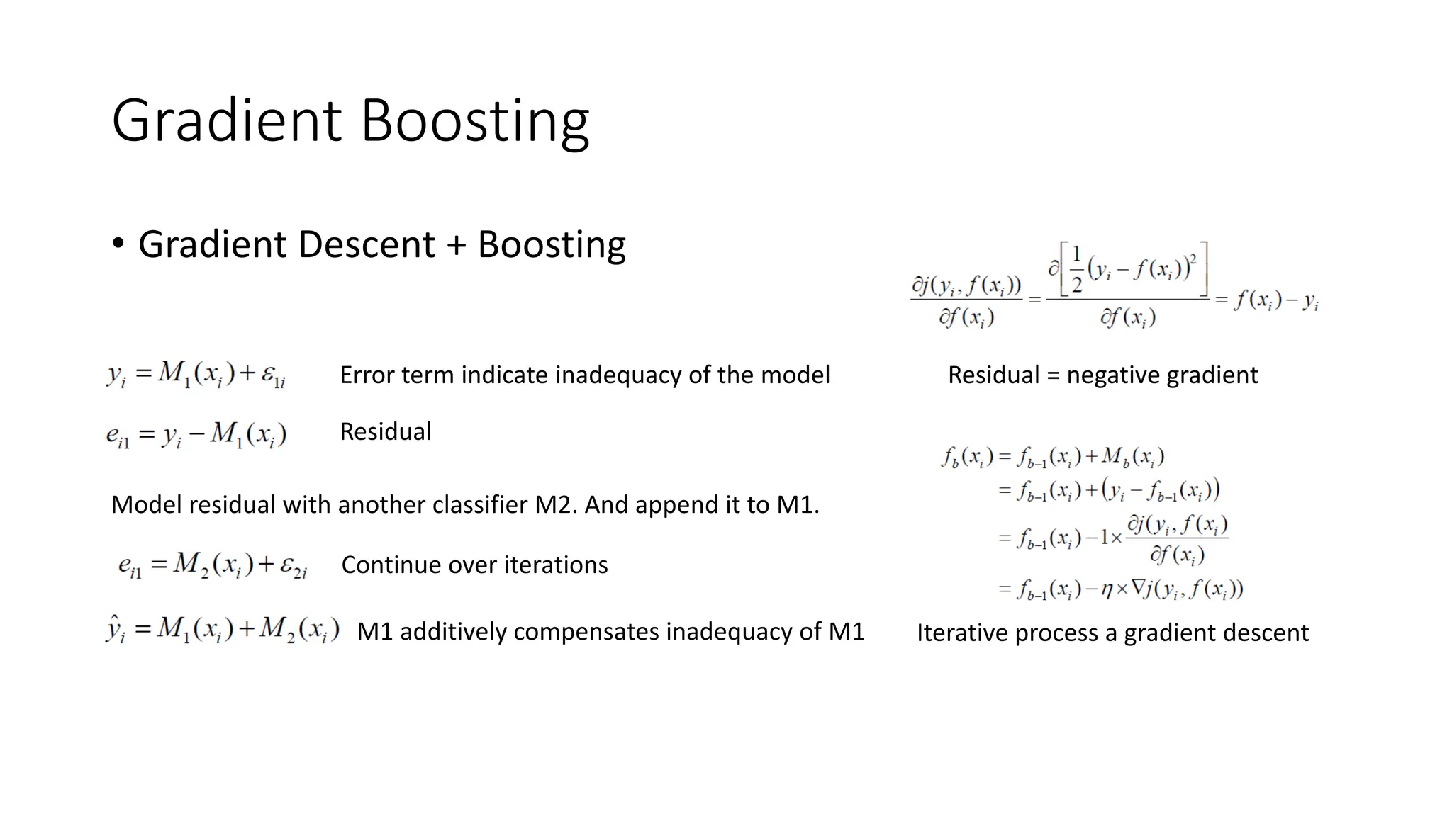
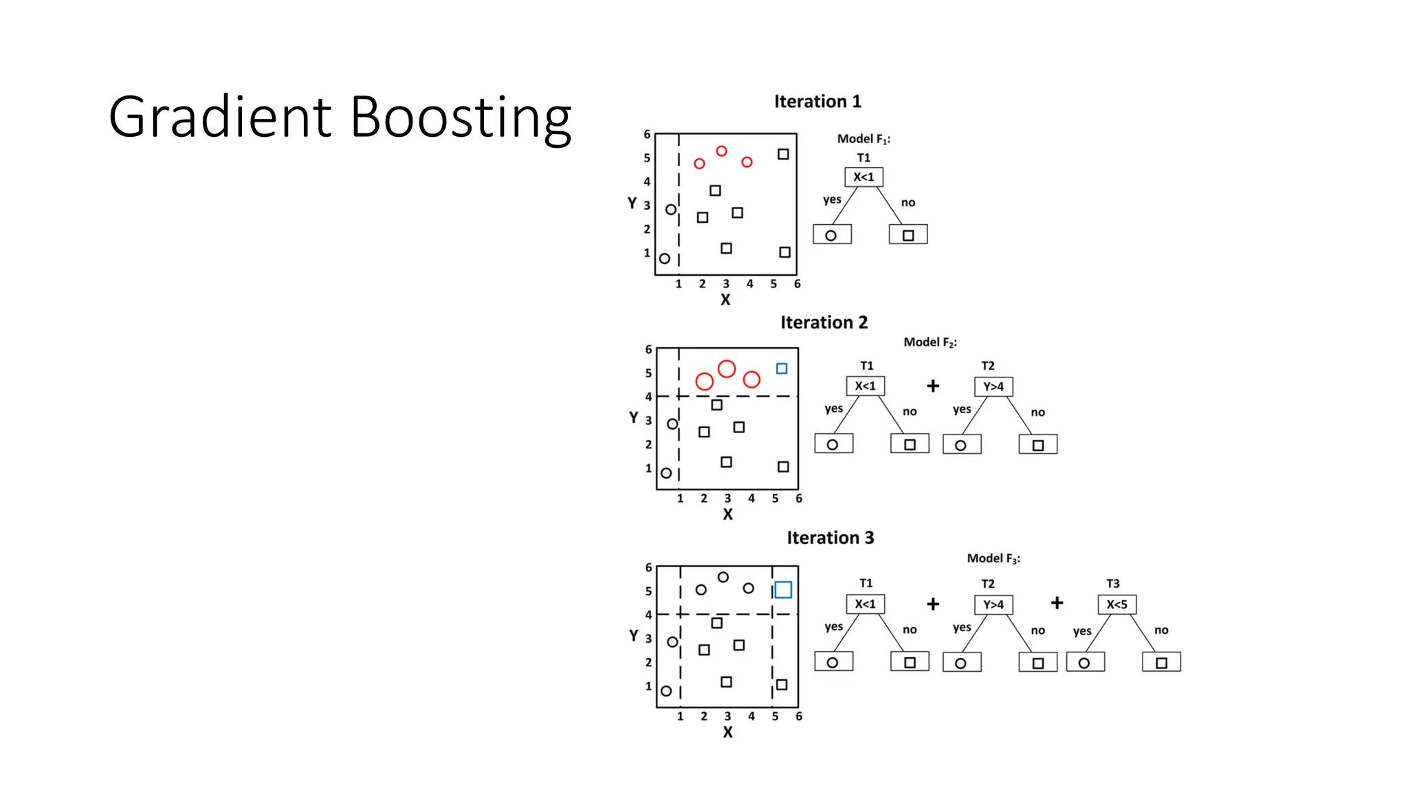
Gradient Boosting
• Gradient Descent + Boosting
Error term indicate inadequacy of the model
Residual
Model residual with another classifier M2. And append it to M1.
Continue over iterations
M1 additively compensates inadequacy of M1
Residual = negative gradient
Iterative process a gradient descent

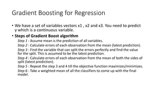
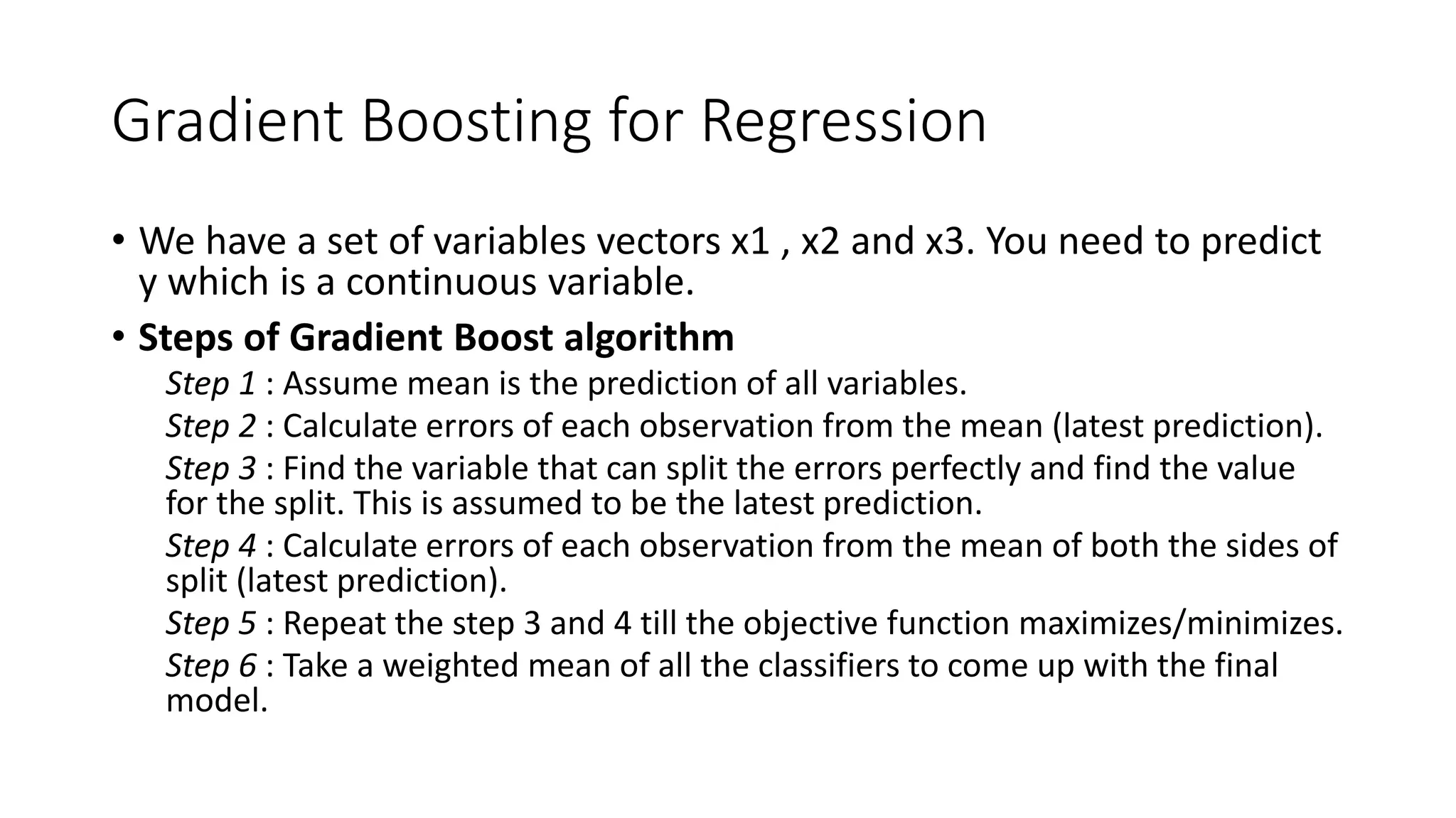
Gradient Boosting for Regression
• We have a set of variables vectors x1 , x2 and x3. You need to predict
y which is a continuous variable.
• Steps of Gradient Boost algorithm
Step 1 : Assume mean is the prediction of all variables.
Step 2 : Calculate errors of each observation from the mean (latest prediction).
Step 3 : Find the variable that can split the errors perfectly and find the value
for the split. This is assumed to be the latest prediction.
Step 4 : Calculate errors of each observation from the mean of both the sides of
split (latest prediction).
Step 5 : Repeat the step 3 and 4 till the objective function maximizes/minimizes.
Step 6 : Take a weighted mean of all the classifiers to come up with the final
model.

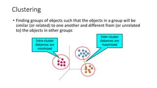
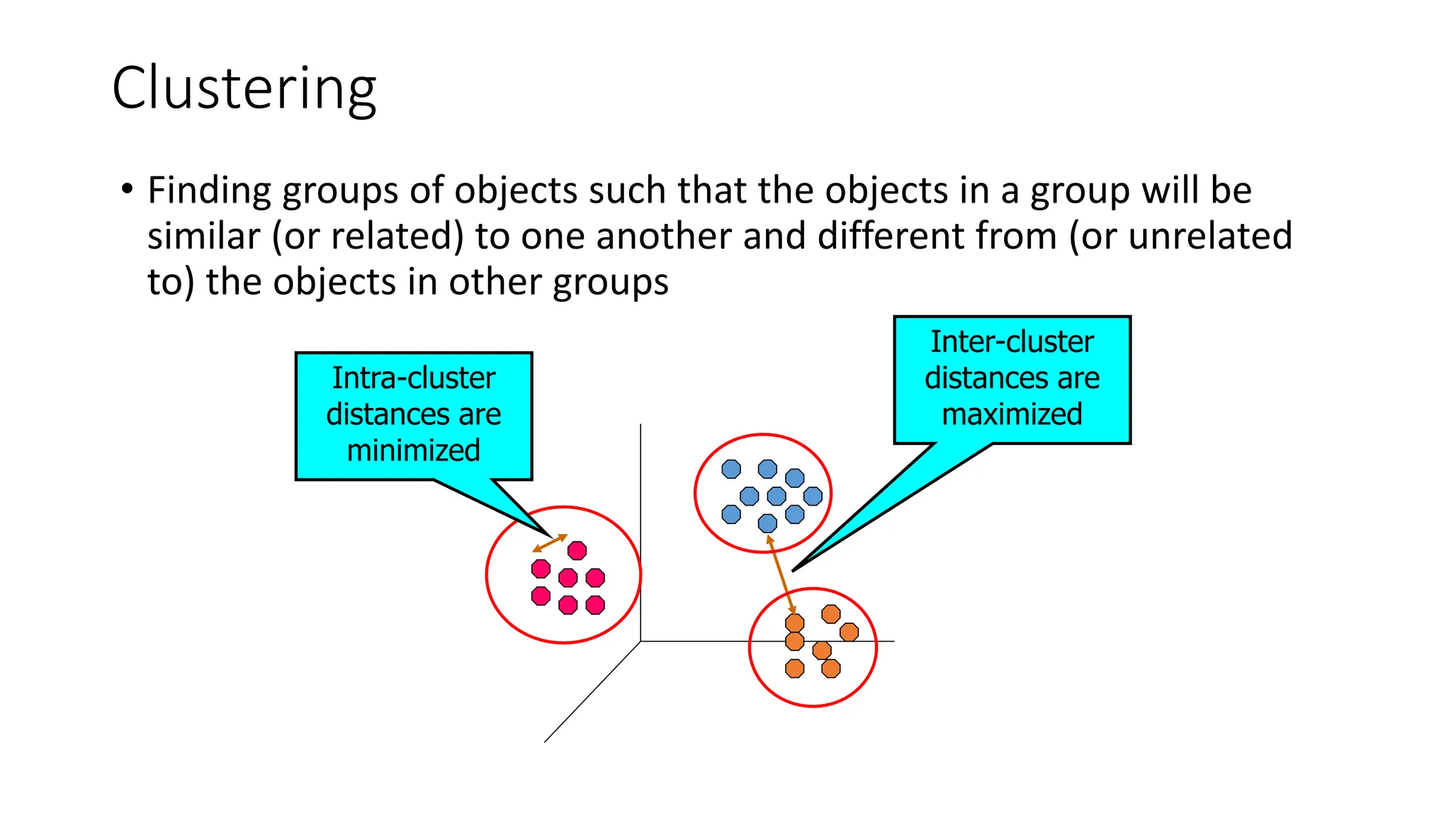
XGBoost: eXtreme Gradient Boosting
• Gradient Boosting + Regularization

Clustering
• Finding groups of objects such that the objects in a group will be
similar (or related) to one another and different from (or unrelated
to) the objects in other groups
Inter-cluster
distances are
maximized
Intra-cluster
distances are
minimized

Clustering Algorithms
p4
p1
p3
p2
p4
p1 p2 p3
Partitional Clustering Hierarchical Clustering

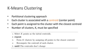
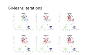
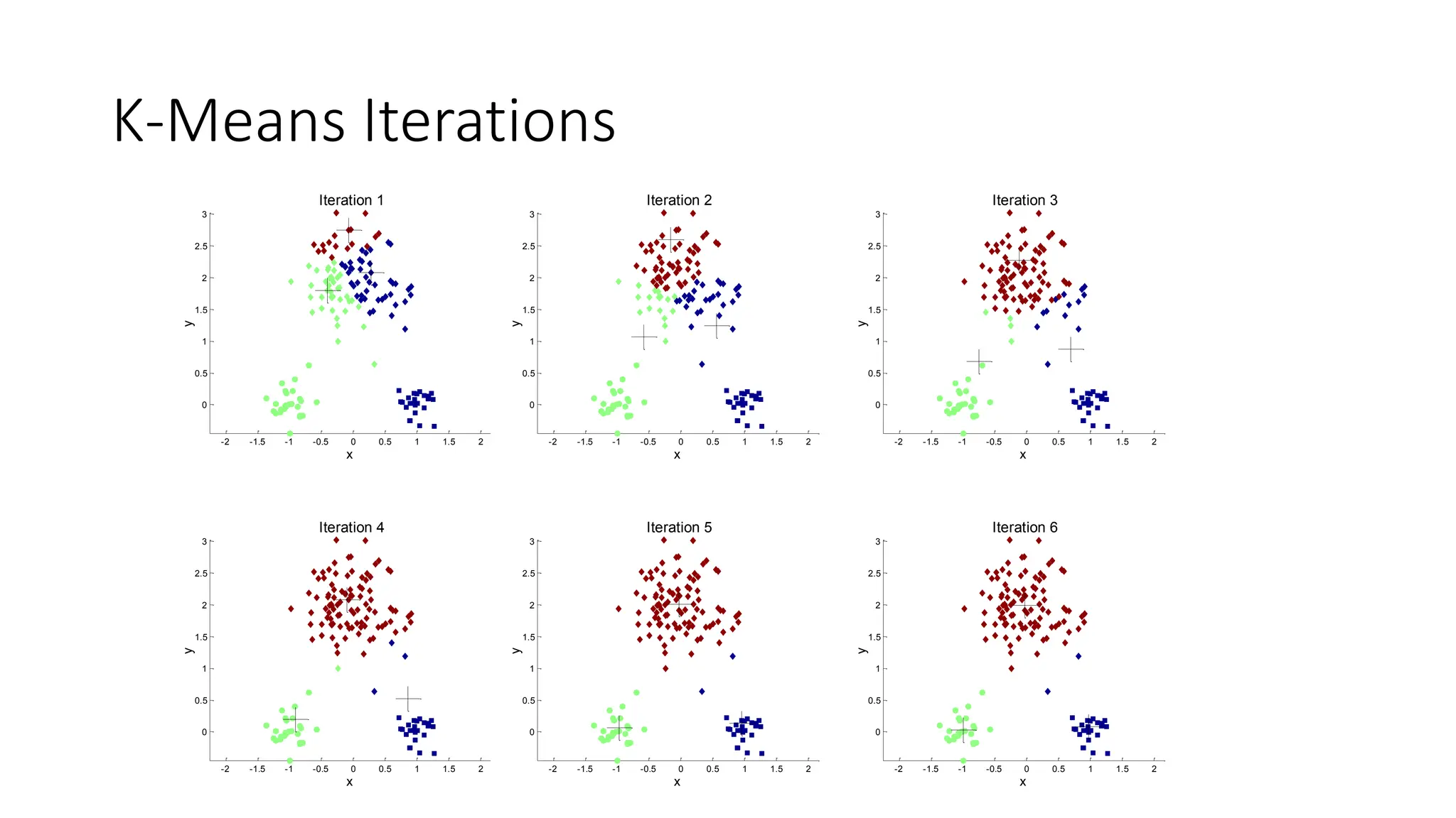
K-Means Clustering
• Partitional clustering approach
• Each cluster is associated with a centroid (center point)
• Each point is assigned to the cluster with the closest centroid
• Number of clusters, K, must be specified

K-Means Iterations
-2 -1.5 -1 -0.5 0 0.5 1 1.5 2
0
0.5
1
1.5
2
2.5
3
x
y
Iteration 1
-2 -1.5 -1 -0.5 0 0.5 1 1.5 2
0
0.5
1
1.5
2
2.5
3
x
y
Iteration 2
-2 -1.5 -1 -0.5 0 0.5 1 1.5 2
0
0.5
1
1.5
2
2.5
3
x
y
Iteration 3
-2 -1.5 -1 -0.5 0 0.5 1 1.5 2
0
0.5
1
1.5
2
2.5
3
x
y
Iteration 4
-2 -1.5 -1 -0.5 0 0.5 1 1.5 2
0
0.5
1
1.5
2
2.5
3
x
y
Iteration 5
-2 -1.5 -1 -0.5 0 0.5 1 1.5 2
0
0.5
1
1.5
2
2.5
3
x
y
Iteration 6

Machine Learning Algorithms Introduction.pdf

More Related Content

Similar to Machine Learning Algorithms Introduction.pdf

Recently uploaded

Machine Learning Algorithms Introduction.pdf