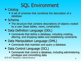
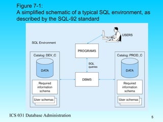
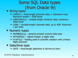
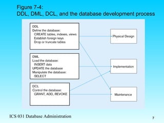
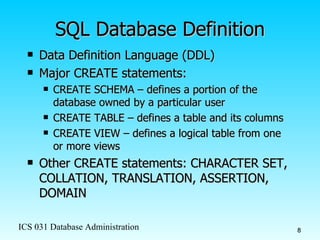
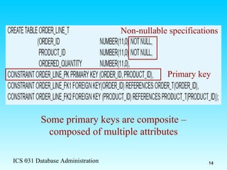
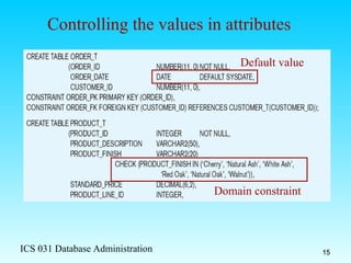
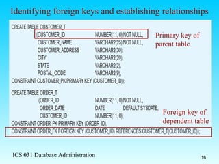
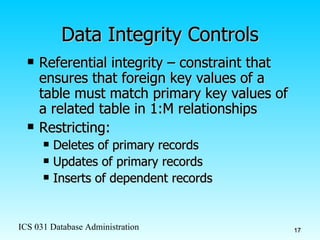
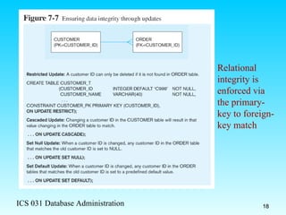
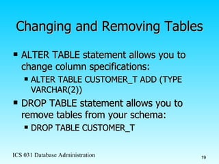
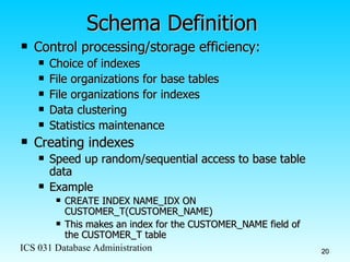
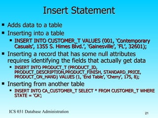
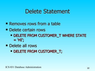
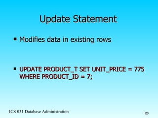
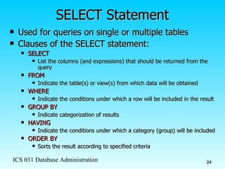
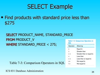
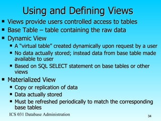
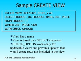
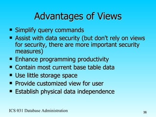
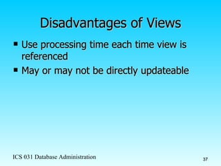
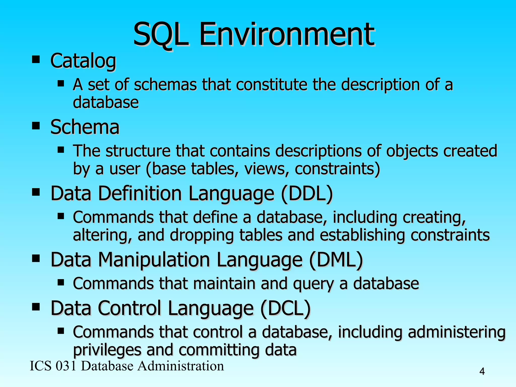
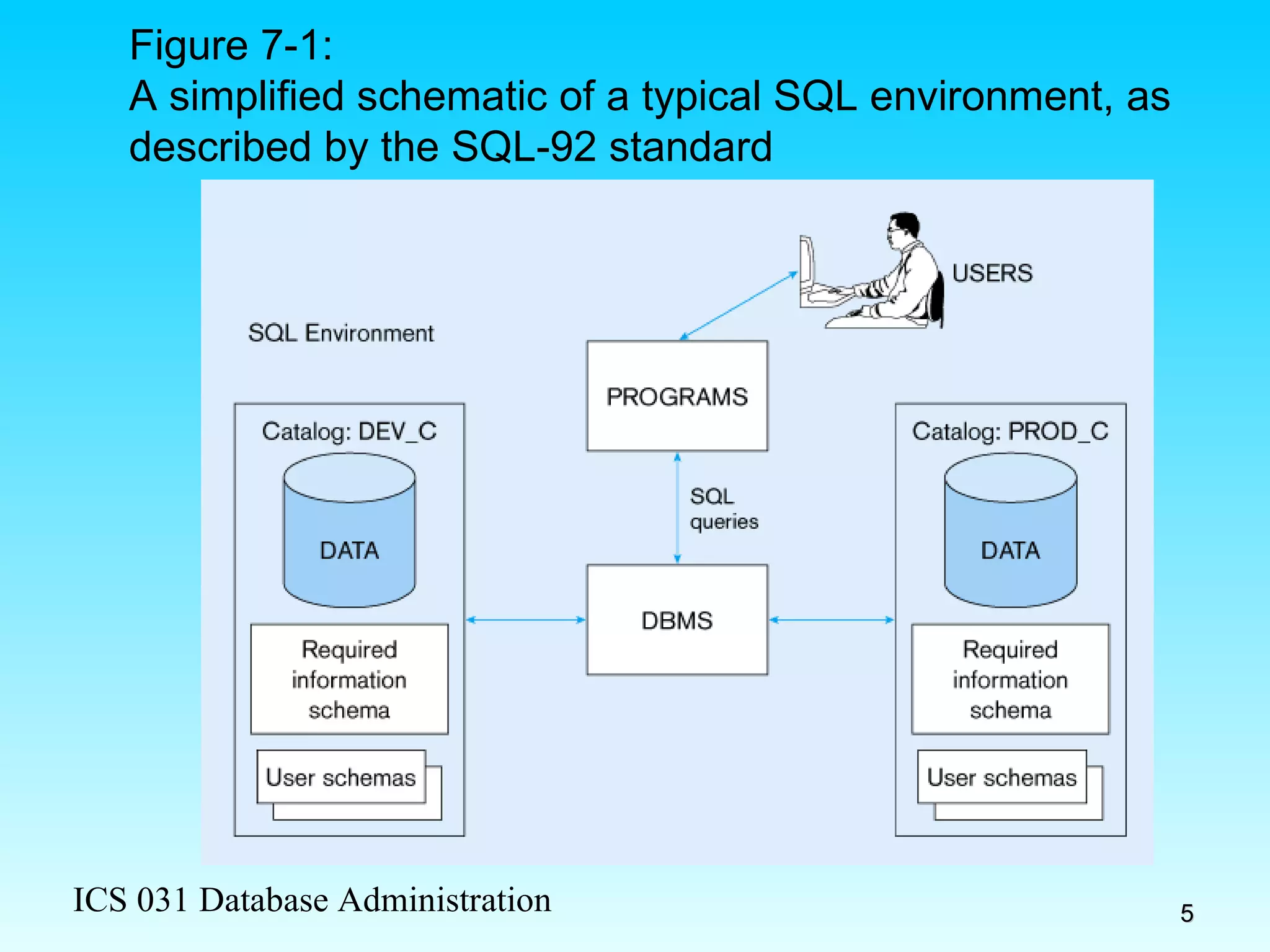
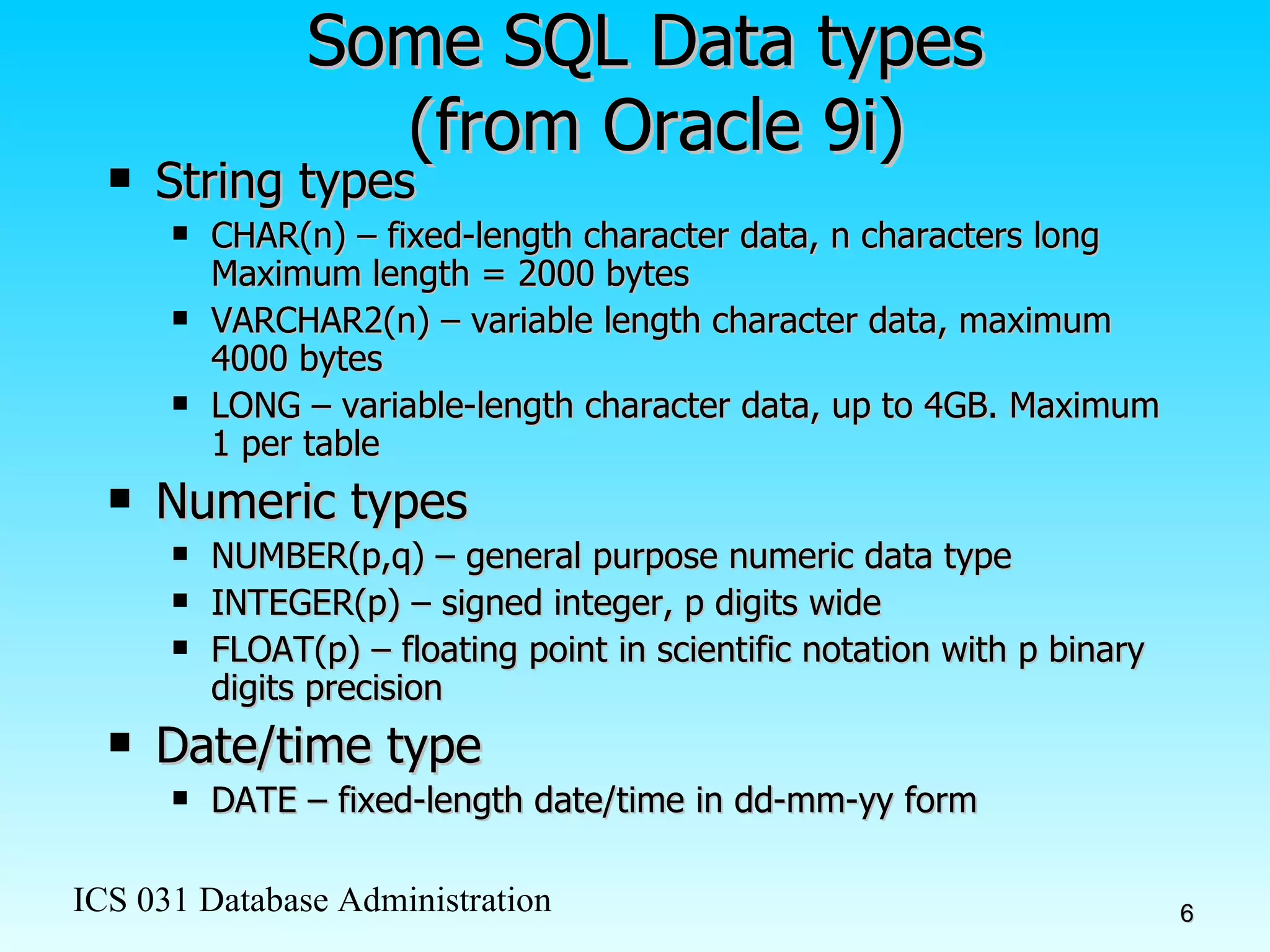
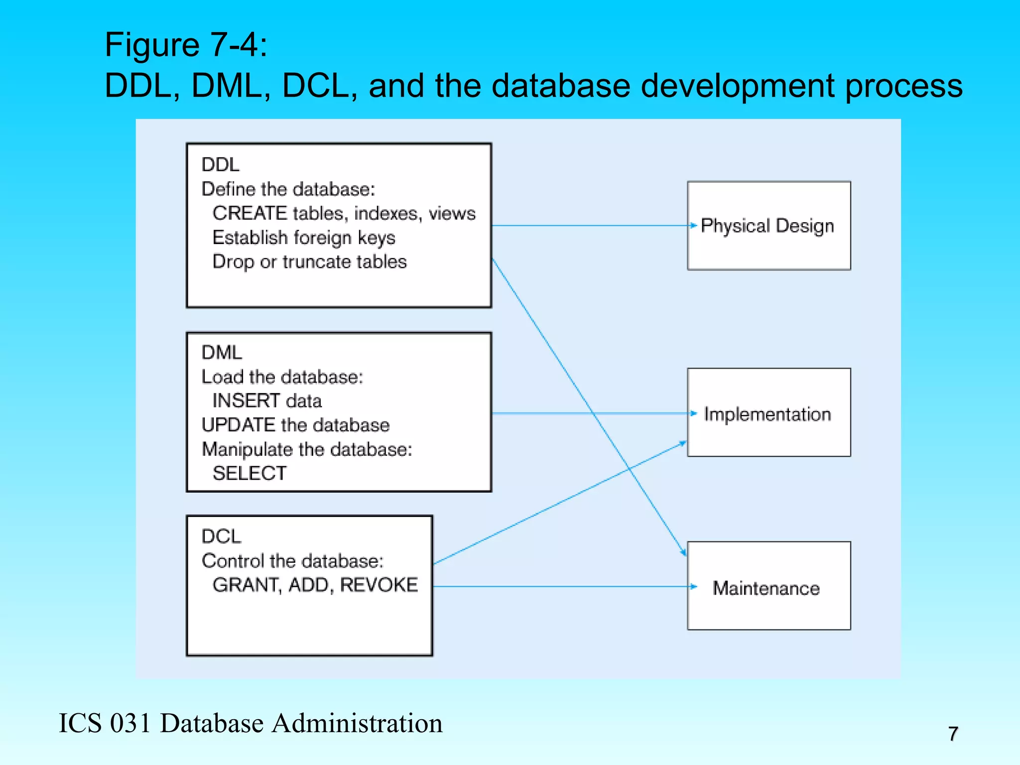
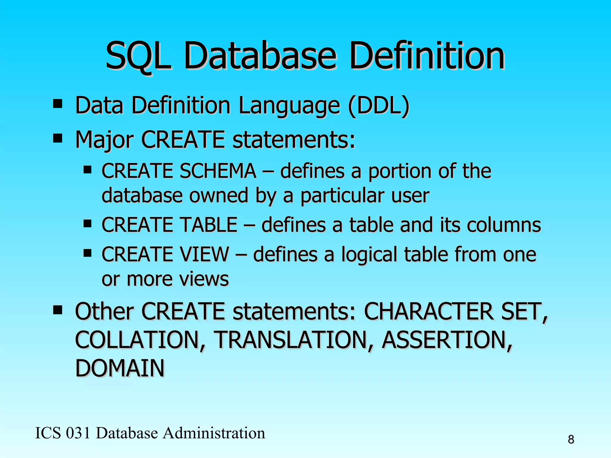
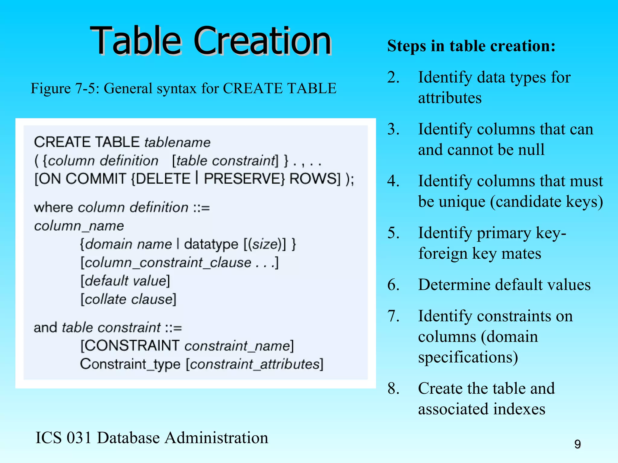
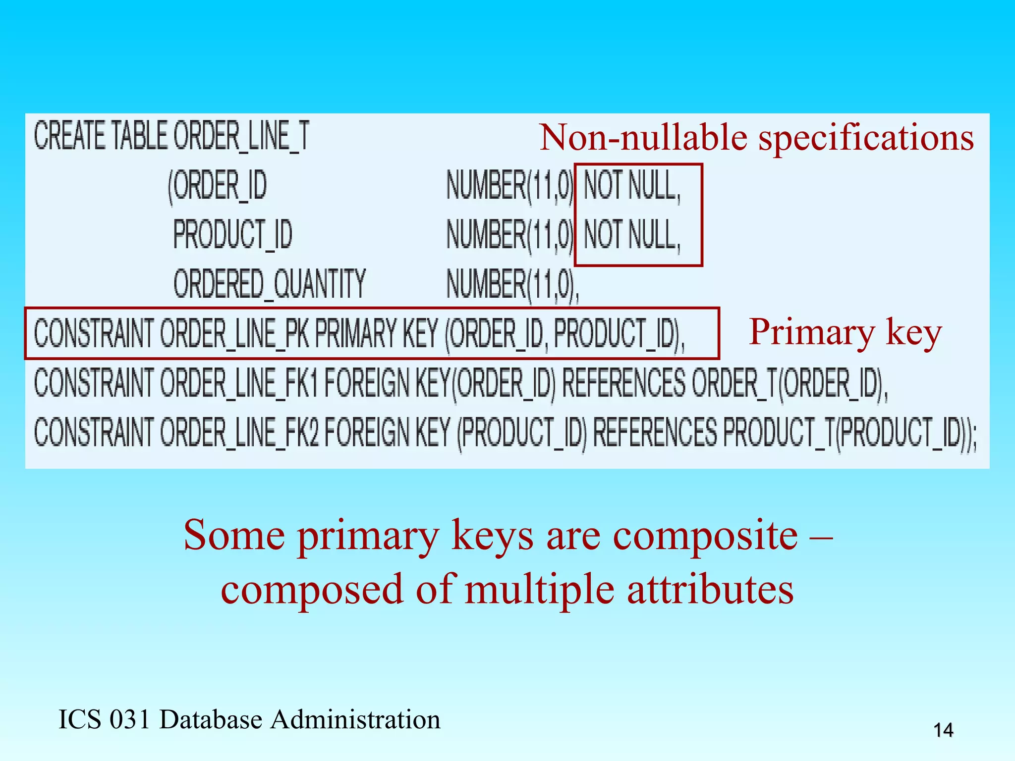
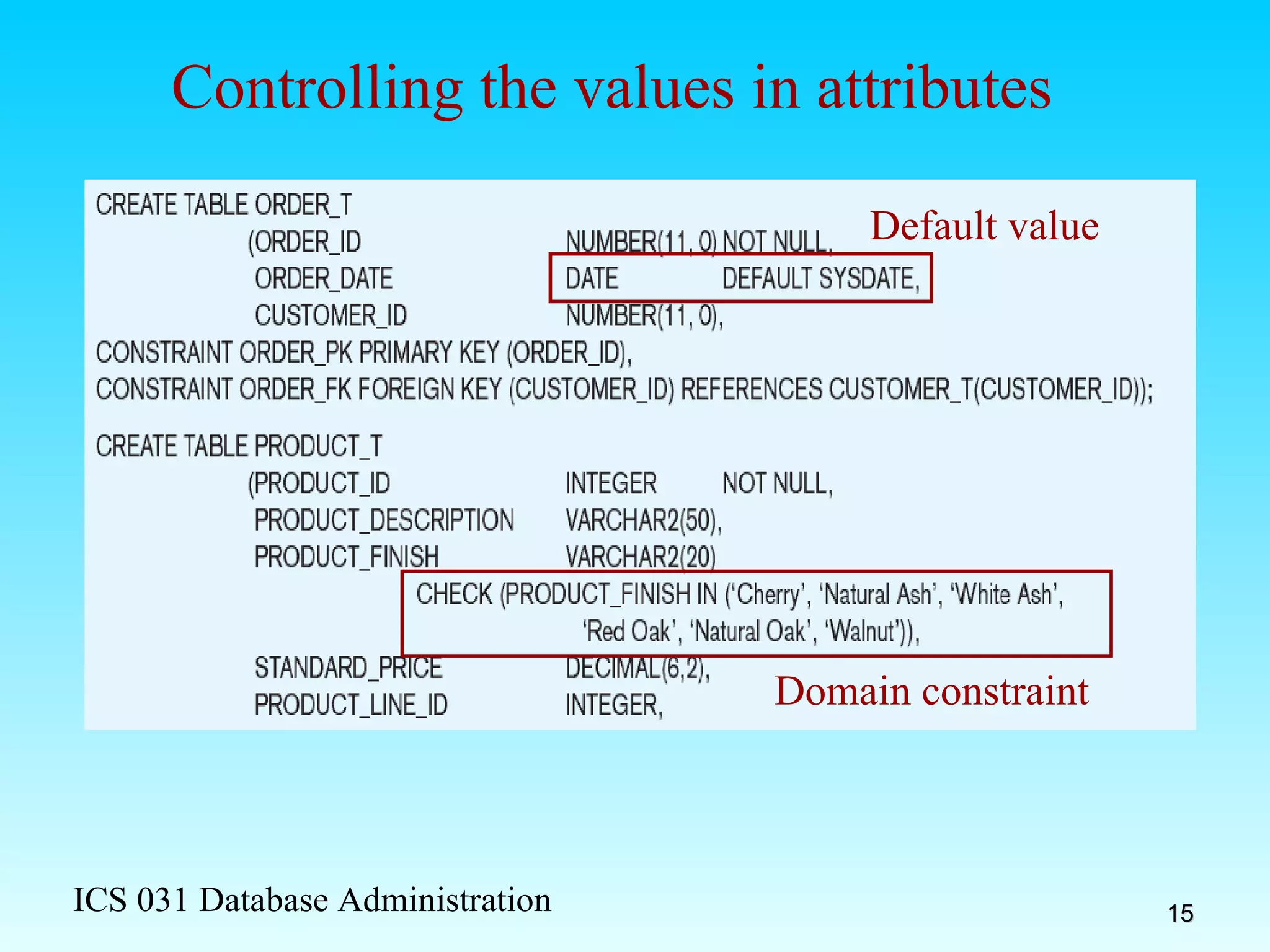
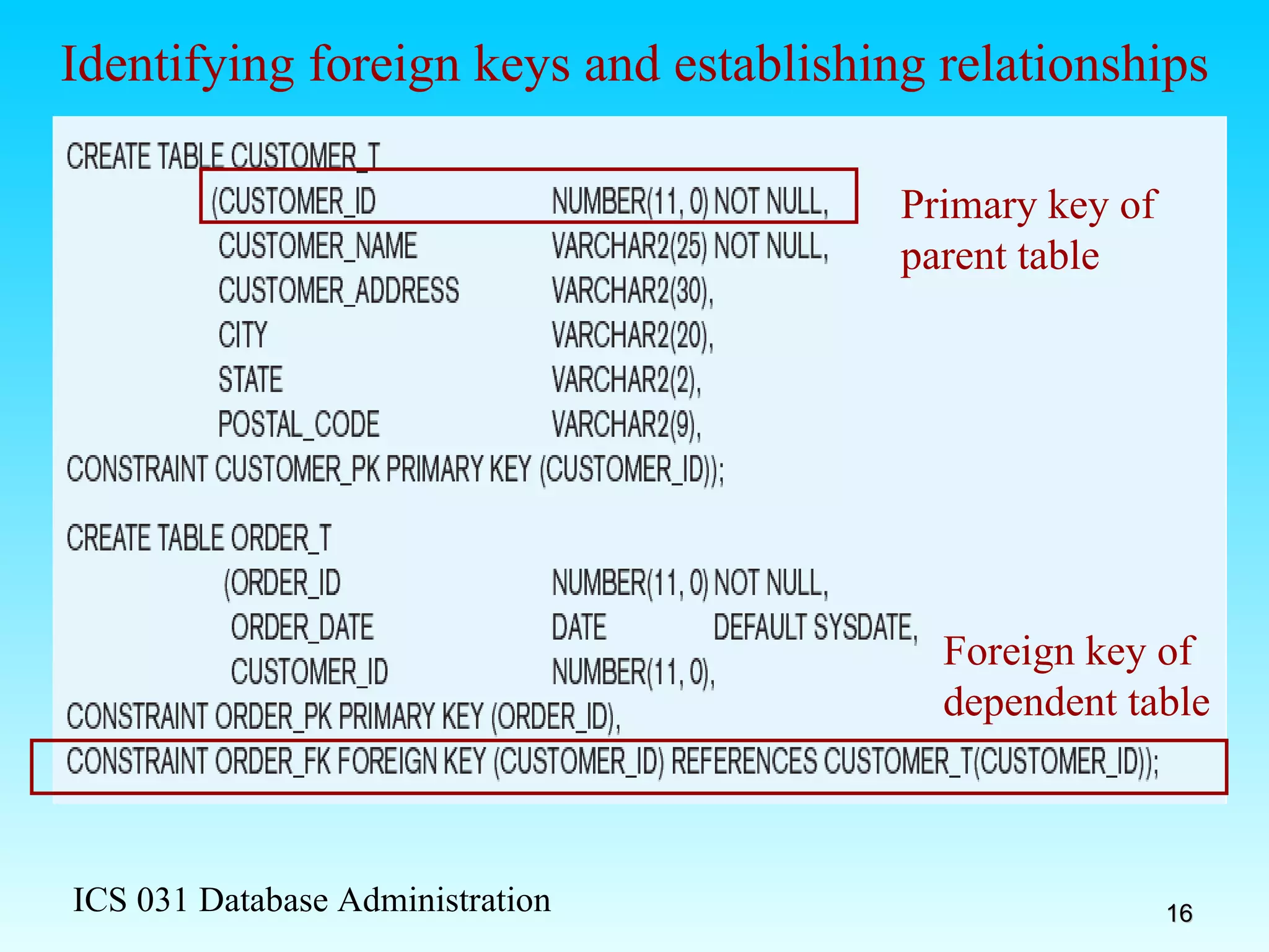
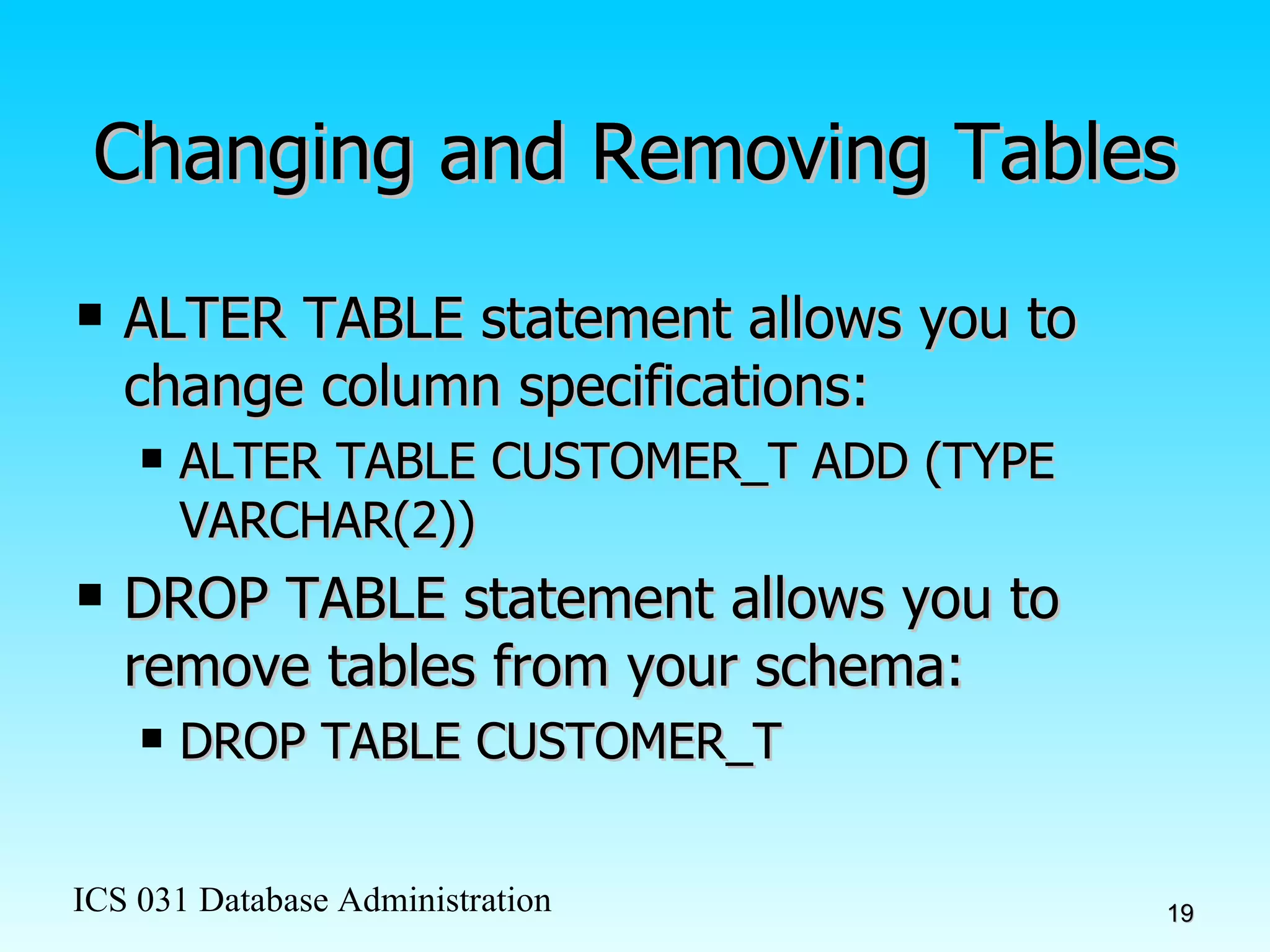
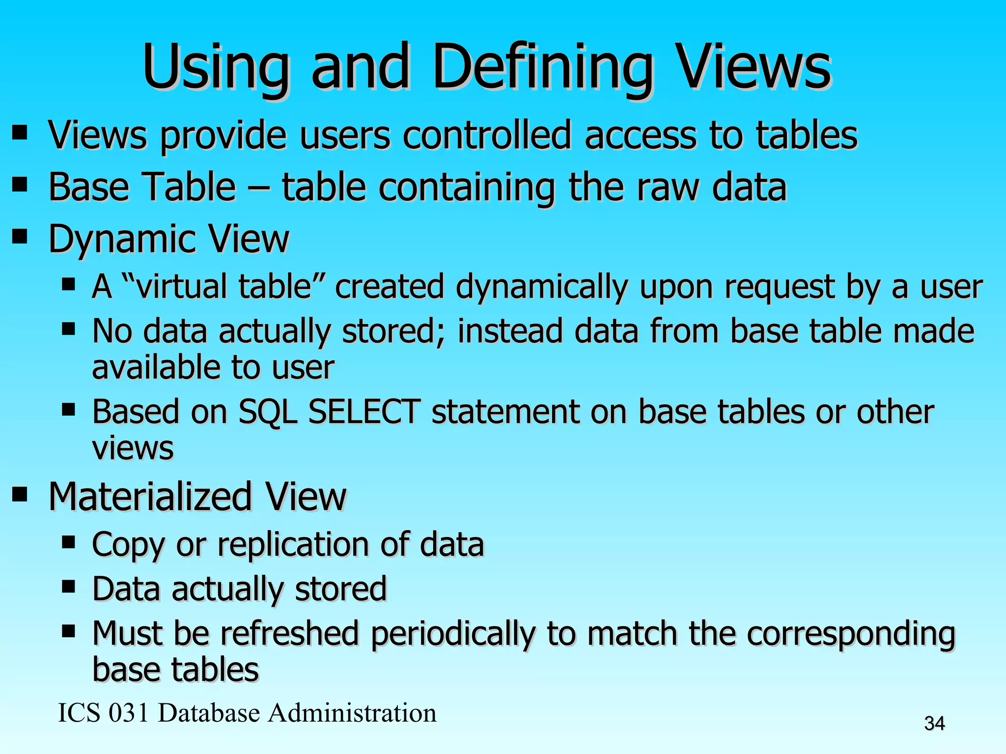
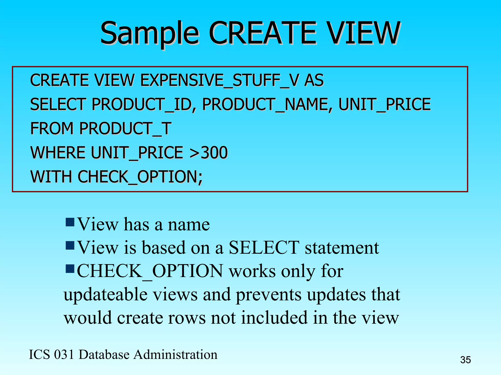
KEMBAR78
Review of SQL | PPT
Review of SQL ICS 031 – Jaweed Yazdani
SQL Overview Structured Query Language The standard for relational database management systems (RDBMS)  SQL-92 and SQL-99 Standards – Purpose: Specify syntax/semantics for data definition and manipulation Define data structures Enable portability Specify minimal (level 1) and complete (level 2) standards Allow for later growth/enhancement to standard
Benefits of a Standardized Relational Language Reduced training costs Productivity Application portability Application longevity Reduced dependence on a single vendor Cross-system communication
SQL Environment Catalog   A set of schemas that constitute the description of a database Schema The structure that contains descriptions of objects created by a user (base tables, views, constraints) Data Definition Language (DDL) Commands that define a database, including creating, altering, and dropping tables and establishing constraints Data Manipulation Language (DML) Commands that maintain and query a database Data Control Language (DCL) Commands that control a database, including administering privileges and committing data
Figure 7-1: A simplified schematic of a typical SQL environment, as described by the SQL-92 standard
Some SQL Data types  (from Oracle 9i) String types CHAR(n) – fixed-length character data, n characters long Maximum length = 2000 bytes VARCHAR2(n) – variable length character data, maximum 4000 bytes LONG – variable-length character data, up to 4GB. Maximum 1 per table Numeric types NUMBER(p,q) – general purpose numeric data type INTEGER(p) – signed integer, p digits wide FLOAT(p) – floating point in scientific notation with p binary digits precision Date/time type DATE – fixed-length date/time in dd-mm-yy form
Figure 7-4:  DDL, DML, DCL, and the database development process
SQL Database Definition Data Definition Language (DDL) Major CREATE statements: CREATE SCHEMA – defines a portion of the database owned by a particular user CREATE TABLE – defines a table and its columns CREATE VIEW – defines a logical table from one or more views Other CREATE statements: CHARACTER SET, COLLATION, TRANSLATION, ASSERTION, DOMAIN
Table Creation Figure 7-5: General syntax for CREATE TABLE Steps in table creation: Identify data types for attributes Identify columns that can and cannot be null Identify columns that must be unique (candidate keys) Identify primary key-foreign key mates Determine default values Identify constraints on columns (domain specifications) Create the table and associated indexes
The following slides create tables for this enterprise data model
Figure 7-6: SQL database definition commands for Pine Valley Furniture Overall table definitions
Defining attributes and their data types
Non-nullable specification Identifying primary key Primary keys can never have NULL values
Non-nullable specifications Primary key Some primary keys are composite – composed of multiple attributes
Default value Domain constraint Controlling the values in attributes
Primary key of  parent table Identifying foreign keys and establishing relationships Foreign key of  dependent table
Data Integrity Controls Referential integrity – constraint that ensures that foreign key values of a table must match primary key values of a related table in 1:M relationships Restricting: Deletes of primary records Updates of primary records Inserts of dependent records
Relational integrity is enforced via the primary-key to foreign-key match
Changing and Removing Tables ALTER TABLE statement allows you to change column specifications: ALTER TABLE CUSTOMER_T ADD (TYPE VARCHAR(2)) DROP TABLE statement allows you to remove tables from your schema: DROP TABLE CUSTOMER_T
Schema Definition Control processing/storage efficiency: Choice of indexes File organizations for base tables File organizations for indexes Data clustering Statistics maintenance Creating indexes Speed up random/sequential access to base table data Example CREATE INDEX NAME_IDX ON CUSTOMER_T(CUSTOMER_NAME) This makes an index for the CUSTOMER_NAME field of the CUSTOMER_T table
Insert Statement Adds data to a table Inserting into a table INSERT INTO CUSTOMER_T VALUES (001, ‘Contemporary Casuals’, 1355 S. Himes Blvd.’, ‘Gainesville’, ‘FL’, 32601); Inserting a record that has some null attributes requires identifying the fields that actually get data INSERT INTO PRODUCT_T (PRODUCT_ID, PRODUCT_DESCRIPTION,PRODUCT_FINISH, STANDARD_PRICE, PRODUCT_ON_HAND) VALUES (1, ‘End Table’, ‘Cherry’, 175, 8); Inserting from another table INSERT INTO CA_CUSTOMER_T SELECT * FROM CUSTOMER_T WHERE STATE = ‘CA’;
Delete Statement Removes rows from a table Delete certain rows DELETE FROM CUSTOMER_T WHERE STATE = ‘HI’; Delete all rows DELETE FROM CUSTOMER_T;
Update Statement Modifies data in existing rows UPDATE PRODUCT_T SET UNIT_PRICE = 775 WHERE PRODUCT_ID = 7;
SELECT Statement Used for queries on single or multiple tables Clauses of the SELECT statement: SELECT List the columns (and expressions) that should be returned from the query FROM Indicate the table(s) or view(s) from which data will be obtained WHERE Indicate the conditions under which a row will be included in the result GROUP BY Indicate categorization of results  HAVING Indicate the conditions under which a category (group) will be included ORDER BY Sorts the result according to specified criteria
Figure 7-8: SQL statement processing order  (adapted from van der Lans, p.100)
SELECT Example Find products with standard price less than $275 SELECT  PRODUCT_NAME, STANDARD_PRICE  FROM  PRODUCT_V  WHERE  STANDARD_PRICE < 275; Table 7-3: Comparison Operators in SQL
SELECT Example using Alias Alias is an alternative column or table name SELECT  CUST .CUSTOMER AS  NAME , CUST.CUSTOMER_ADDRESS  FROM CUSTOMER_V  CUST WHERE  NAME  = ‘Home Furnishings’;
SELECT Example  Using a Function Using the COUNT  aggregate function  to find totals SELECT  COUNT(*)  FROM ORDER_LINE_V WHERE ORDER_ID = 1004; Note: with aggregate functions you can’t have single-valued columns included in the SELECT clause
SELECT Example – Boolean Operators AND ,  OR , and  NOT  Operators for customizing conditions in WHERE clause SELECT PRODUCT_DESCRIPTION, PRODUCT_FINISH, STANDARD_PRICE FROM PRODUCT_V WHERE (PRODUCT_DESCRIPTION  LIKE  ‘ % Desk’ OR  PRODUCT_DESCRIPTION  LIKE  ‘ % Table’)  AND  UNIT_PRICE > 300; Note: the LIKE operator allows you to compare strings using wildcards. For example, the % wildcard in ‘%Desk’  indicates that all strings that have any number of characters preceding the word “Desk” will be allowed
SELECT Example –  Sorting Results with the ORDER BY Clause Sort the results first by STATE, and within a state by CUSTOMER_NAME SELECT CUSTOMER_NAME, CITY, STATE FROM CUSTOMER_V WHERE STATE  IN  (‘FL’, ‘TX’, ‘CA’, ‘HI’) ORDER BY STATE, CUSTOMER_NAME; Note: the IN operator in this example allows you to include rows whose STATE value is either FL, TX, CA, or HI. It is more efficient than separate OR conditions
SELECT Example –  Categorizing Results Using the GROUP BY Clause For use with aggregate functions Scalar aggregate : single value returned from SQL query with aggregate function Vector aggregate : multiple values returned from SQL query with aggregate function (via GROUP BY) SELECT STATE, COUNT(STATE)  FROM CUSTOMER_V GROUP BY  STATE; Note: you can use single-value fields with aggregate functions if they are included in the GROUP BY clause
SELECT Example –  Qualifying Results by Categories  Using the HAVING Clause For use with GROUP BY SELECT STATE, COUNT(STATE)  FROM CUSTOMER_V GROUP BY STATE HAVING  COUNT(STATE) > 1; Like a WHERE clause, but it operates on groups (categories), not on individual rows. Here, only those groups with total numbers greater than 1 will be included in final result
Figure 7-8: SQL statement processing order  (adapted from van der Lans, p.100)
Using and Defining Views Views provide users controlled access to tables Base Table – table containing the raw data Dynamic View A “virtual table” created dynamically upon request by a user  No data actually stored; instead data from base table made available to user Based on SQL SELECT statement on base tables or other views Materialized View Copy or replication of data Data actually stored Must be refreshed periodically to match the corresponding base tables
Sample CREATE VIEW CREATE VIEW EXPENSIVE_STUFF_V AS SELECT PRODUCT_ID, PRODUCT_NAME, UNIT_PRICE FROM PRODUCT_T WHERE UNIT_PRICE >300 WITH CHECK_OPTION; View has a name View is based on a SELECT statement CHECK_OPTION works only for updateable views and prevents updates that would create rows not included in the view
Advantages of Views Simplify query commands Assist with data security (but don't rely on views for security, there are more important security measures) Enhance programming productivity Contain most current base table data Use little storage space Provide customized view for user Establish physical data independence
Disadvantages of Views Use processing time each time view is referenced May or may not be directly updateable

Review of SQL

  • 1.
    Review of SQLICS 031 – Jaweed Yazdani
  • 2.
    SQL Overview StructuredQuery Language The standard for relational database management systems (RDBMS) SQL-92 and SQL-99 Standards – Purpose: Specify syntax/semantics for data definition and manipulation Define data structures Enable portability Specify minimal (level 1) and complete (level 2) standards Allow for later growth/enhancement to standard
  • 3.
    Benefits of aStandardized Relational Language Reduced training costs Productivity Application portability Application longevity Reduced dependence on a single vendor Cross-system communication
  • 4.
    SQL Environment Catalog A set of schemas that constitute the description of a database Schema The structure that contains descriptions of objects created by a user (base tables, views, constraints) Data Definition Language (DDL) Commands that define a database, including creating, altering, and dropping tables and establishing constraints Data Manipulation Language (DML) Commands that maintain and query a database Data Control Language (DCL) Commands that control a database, including administering privileges and committing data
  • 5.
    Figure 7-1: Asimplified schematic of a typical SQL environment, as described by the SQL-92 standard
  • 6.
    Some SQL Datatypes (from Oracle 9i) String types CHAR(n) – fixed-length character data, n characters long Maximum length = 2000 bytes VARCHAR2(n) – variable length character data, maximum 4000 bytes LONG – variable-length character data, up to 4GB. Maximum 1 per table Numeric types NUMBER(p,q) – general purpose numeric data type INTEGER(p) – signed integer, p digits wide FLOAT(p) – floating point in scientific notation with p binary digits precision Date/time type DATE – fixed-length date/time in dd-mm-yy form
  • 7.
    Figure 7-4: DDL, DML, DCL, and the database development process
  • 8.
    SQL Database DefinitionData Definition Language (DDL) Major CREATE statements: CREATE SCHEMA – defines a portion of the database owned by a particular user CREATE TABLE – defines a table and its columns CREATE VIEW – defines a logical table from one or more views Other CREATE statements: CHARACTER SET, COLLATION, TRANSLATION, ASSERTION, DOMAIN
  • 9.
    Table Creation Figure7-5: General syntax for CREATE TABLE Steps in table creation: Identify data types for attributes Identify columns that can and cannot be null Identify columns that must be unique (candidate keys) Identify primary key-foreign key mates Determine default values Identify constraints on columns (domain specifications) Create the table and associated indexes
  • 10.
    The following slidescreate tables for this enterprise data model
  • 11.
    Figure 7-6: SQLdatabase definition commands for Pine Valley Furniture Overall table definitions
  • 12.
    Defining attributes andtheir data types
  • 13.
    Non-nullable specification Identifyingprimary key Primary keys can never have NULL values
  • 14.
    Non-nullable specifications Primarykey Some primary keys are composite – composed of multiple attributes
  • 15.
    Default value Domainconstraint Controlling the values in attributes
  • 16.
    Primary key of parent table Identifying foreign keys and establishing relationships Foreign key of dependent table
  • 17.
    Data Integrity ControlsReferential integrity – constraint that ensures that foreign key values of a table must match primary key values of a related table in 1:M relationships Restricting: Deletes of primary records Updates of primary records Inserts of dependent records
  • 18.
    Relational integrity isenforced via the primary-key to foreign-key match
  • 19.
    Changing and RemovingTables ALTER TABLE statement allows you to change column specifications: ALTER TABLE CUSTOMER_T ADD (TYPE VARCHAR(2)) DROP TABLE statement allows you to remove tables from your schema: DROP TABLE CUSTOMER_T
  • 20.
    Schema Definition Controlprocessing/storage efficiency: Choice of indexes File organizations for base tables File organizations for indexes Data clustering Statistics maintenance Creating indexes Speed up random/sequential access to base table data Example CREATE INDEX NAME_IDX ON CUSTOMER_T(CUSTOMER_NAME) This makes an index for the CUSTOMER_NAME field of the CUSTOMER_T table
  • 21.
    Insert Statement Addsdata to a table Inserting into a table INSERT INTO CUSTOMER_T VALUES (001, ‘Contemporary Casuals’, 1355 S. Himes Blvd.’, ‘Gainesville’, ‘FL’, 32601); Inserting a record that has some null attributes requires identifying the fields that actually get data INSERT INTO PRODUCT_T (PRODUCT_ID, PRODUCT_DESCRIPTION,PRODUCT_FINISH, STANDARD_PRICE, PRODUCT_ON_HAND) VALUES (1, ‘End Table’, ‘Cherry’, 175, 8); Inserting from another table INSERT INTO CA_CUSTOMER_T SELECT * FROM CUSTOMER_T WHERE STATE = ‘CA’;
  • 22.
    Delete Statement Removesrows from a table Delete certain rows DELETE FROM CUSTOMER_T WHERE STATE = ‘HI’; Delete all rows DELETE FROM CUSTOMER_T;
  • 23.
    Update Statement Modifiesdata in existing rows UPDATE PRODUCT_T SET UNIT_PRICE = 775 WHERE PRODUCT_ID = 7;
  • 24.
    SELECT Statement Usedfor queries on single or multiple tables Clauses of the SELECT statement: SELECT List the columns (and expressions) that should be returned from the query FROM Indicate the table(s) or view(s) from which data will be obtained WHERE Indicate the conditions under which a row will be included in the result GROUP BY Indicate categorization of results HAVING Indicate the conditions under which a category (group) will be included ORDER BY Sorts the result according to specified criteria
  • 25.
    Figure 7-8: SQLstatement processing order (adapted from van der Lans, p.100)
  • 26.
    SELECT Example Findproducts with standard price less than $275 SELECT PRODUCT_NAME, STANDARD_PRICE FROM PRODUCT_V WHERE STANDARD_PRICE < 275; Table 7-3: Comparison Operators in SQL
  • 27.
    SELECT Example usingAlias Alias is an alternative column or table name SELECT CUST .CUSTOMER AS NAME , CUST.CUSTOMER_ADDRESS FROM CUSTOMER_V CUST WHERE NAME = ‘Home Furnishings’;
  • 28.
    SELECT Example Using a Function Using the COUNT aggregate function to find totals SELECT COUNT(*) FROM ORDER_LINE_V WHERE ORDER_ID = 1004; Note: with aggregate functions you can’t have single-valued columns included in the SELECT clause
  • 29.
    SELECT Example –Boolean Operators AND , OR , and NOT Operators for customizing conditions in WHERE clause SELECT PRODUCT_DESCRIPTION, PRODUCT_FINISH, STANDARD_PRICE FROM PRODUCT_V WHERE (PRODUCT_DESCRIPTION LIKE ‘ % Desk’ OR PRODUCT_DESCRIPTION LIKE ‘ % Table’) AND UNIT_PRICE > 300; Note: the LIKE operator allows you to compare strings using wildcards. For example, the % wildcard in ‘%Desk’ indicates that all strings that have any number of characters preceding the word “Desk” will be allowed
  • 30.
    SELECT Example – Sorting Results with the ORDER BY Clause Sort the results first by STATE, and within a state by CUSTOMER_NAME SELECT CUSTOMER_NAME, CITY, STATE FROM CUSTOMER_V WHERE STATE IN (‘FL’, ‘TX’, ‘CA’, ‘HI’) ORDER BY STATE, CUSTOMER_NAME; Note: the IN operator in this example allows you to include rows whose STATE value is either FL, TX, CA, or HI. It is more efficient than separate OR conditions
  • 31.
    SELECT Example – Categorizing Results Using the GROUP BY Clause For use with aggregate functions Scalar aggregate : single value returned from SQL query with aggregate function Vector aggregate : multiple values returned from SQL query with aggregate function (via GROUP BY) SELECT STATE, COUNT(STATE) FROM CUSTOMER_V GROUP BY STATE; Note: you can use single-value fields with aggregate functions if they are included in the GROUP BY clause
  • 32.
    SELECT Example – Qualifying Results by Categories Using the HAVING Clause For use with GROUP BY SELECT STATE, COUNT(STATE) FROM CUSTOMER_V GROUP BY STATE HAVING COUNT(STATE) > 1; Like a WHERE clause, but it operates on groups (categories), not on individual rows. Here, only those groups with total numbers greater than 1 will be included in final result
  • 33.
    Figure 7-8: SQLstatement processing order (adapted from van der Lans, p.100)
  • 34.
    Using and DefiningViews Views provide users controlled access to tables Base Table – table containing the raw data Dynamic View A “virtual table” created dynamically upon request by a user No data actually stored; instead data from base table made available to user Based on SQL SELECT statement on base tables or other views Materialized View Copy or replication of data Data actually stored Must be refreshed periodically to match the corresponding base tables
  • 35.
    Sample CREATE VIEWCREATE VIEW EXPENSIVE_STUFF_V AS SELECT PRODUCT_ID, PRODUCT_NAME, UNIT_PRICE FROM PRODUCT_T WHERE UNIT_PRICE >300 WITH CHECK_OPTION; View has a name View is based on a SELECT statement CHECK_OPTION works only for updateable views and prevents updates that would create rows not included in the view
  • 36.
    Advantages of ViewsSimplify query commands Assist with data security (but don't rely on views for security, there are more important security measures) Enhance programming productivity Contain most current base table data Use little storage space Provide customized view for user Establish physical data independence
  • 37.
    Disadvantages of ViewsUse processing time each time view is referenced May or may not be directly updateable