Download to read offline

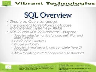
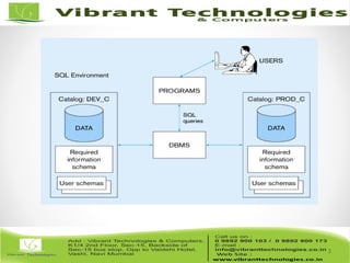
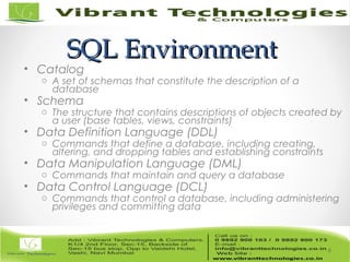
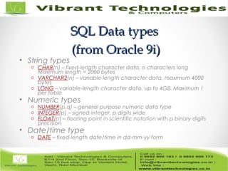
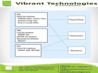
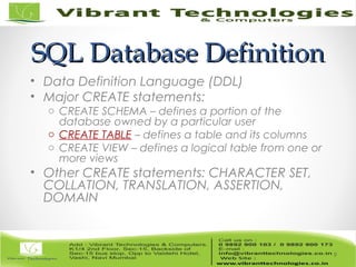
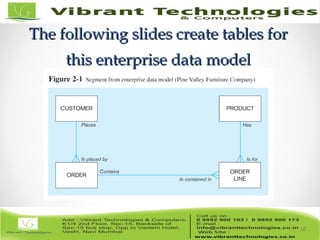
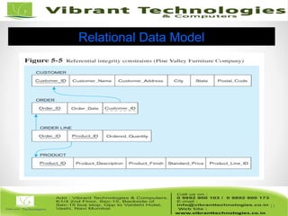
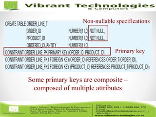

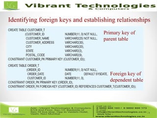
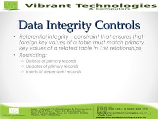
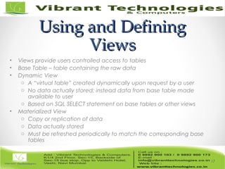
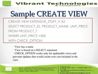


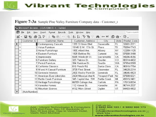
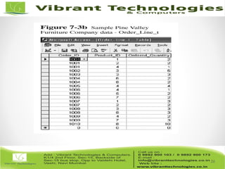
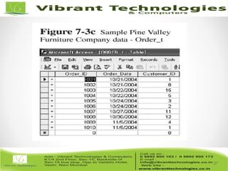
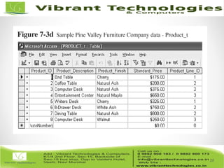

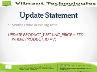
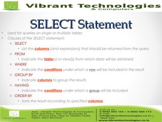
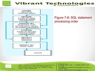

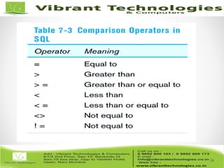
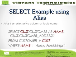
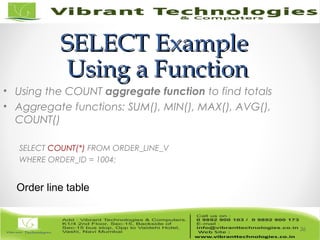
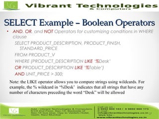
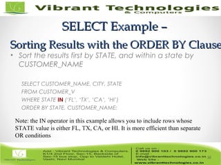

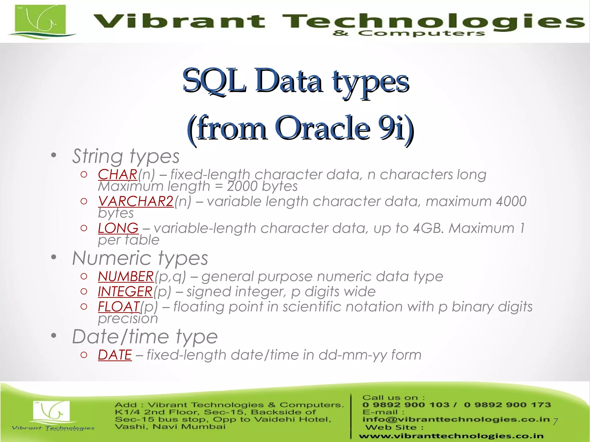
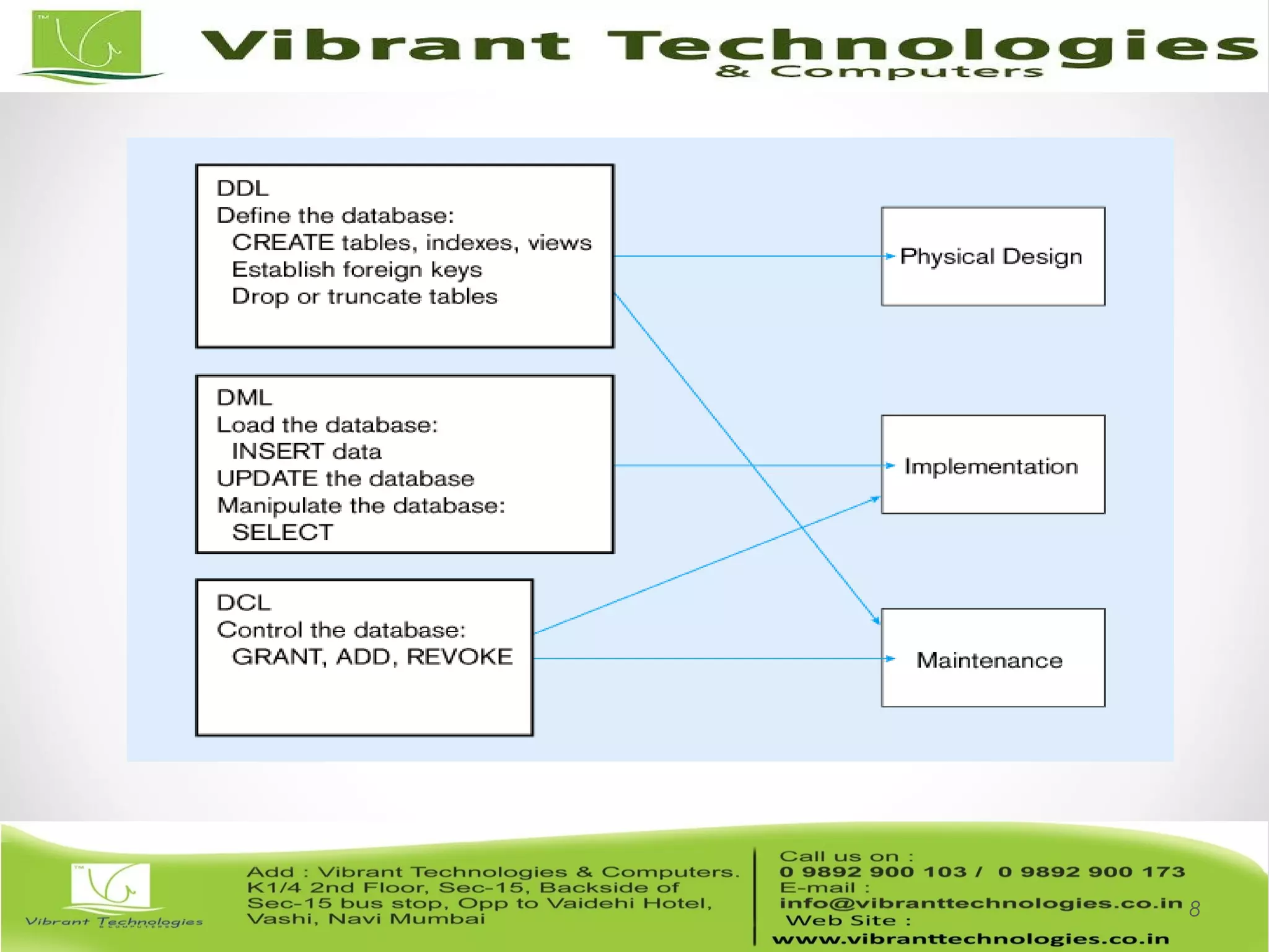
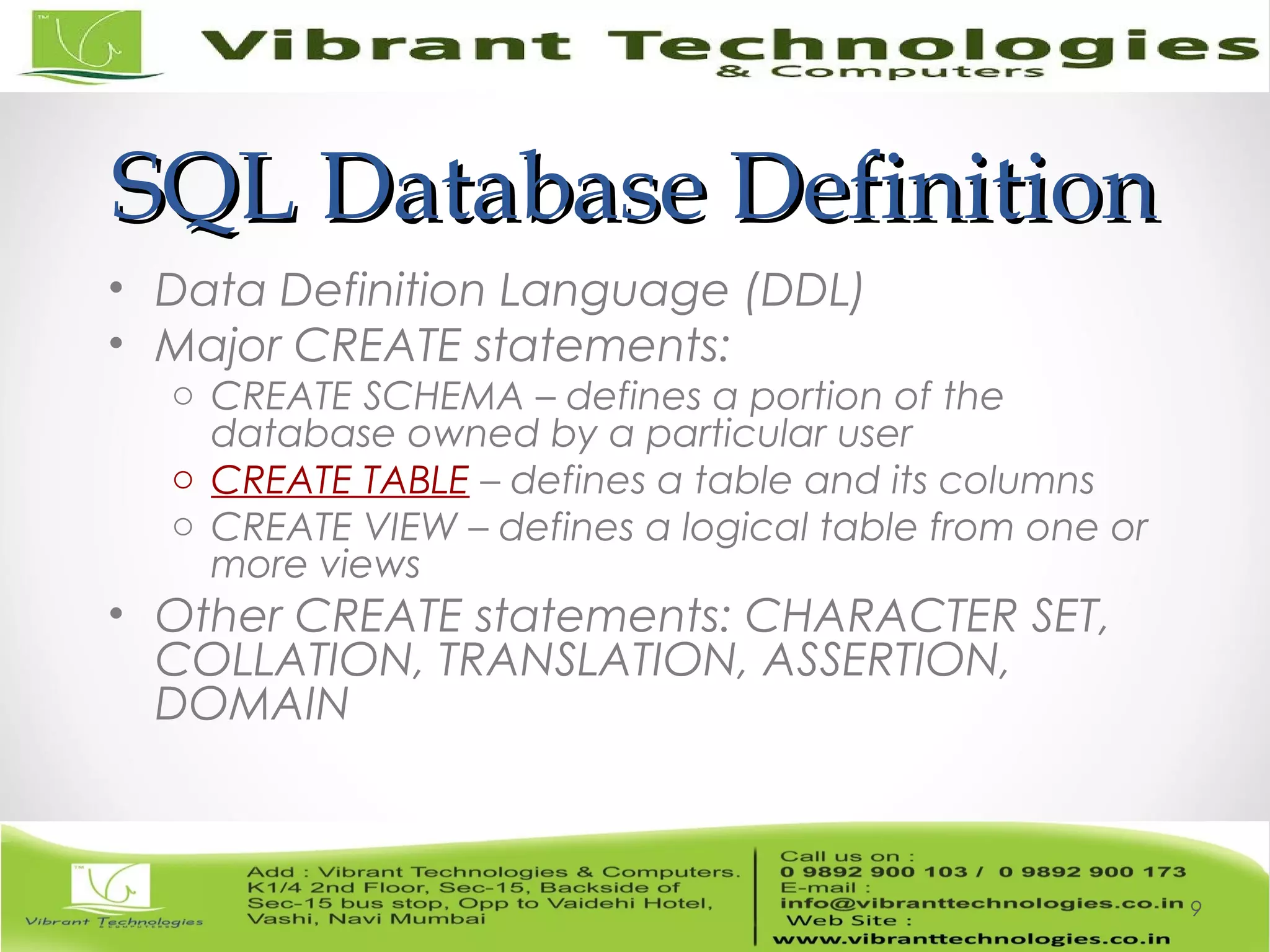
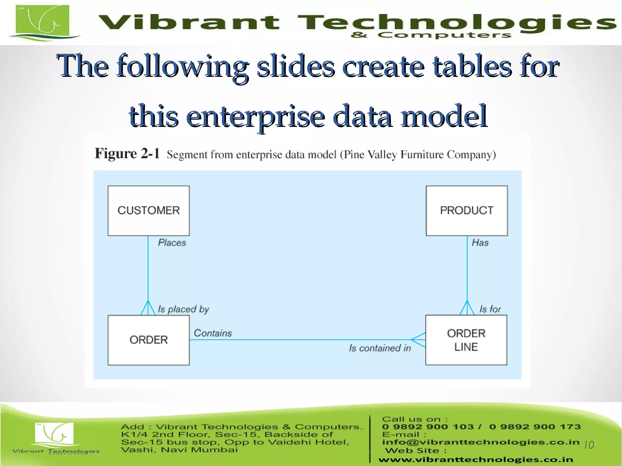
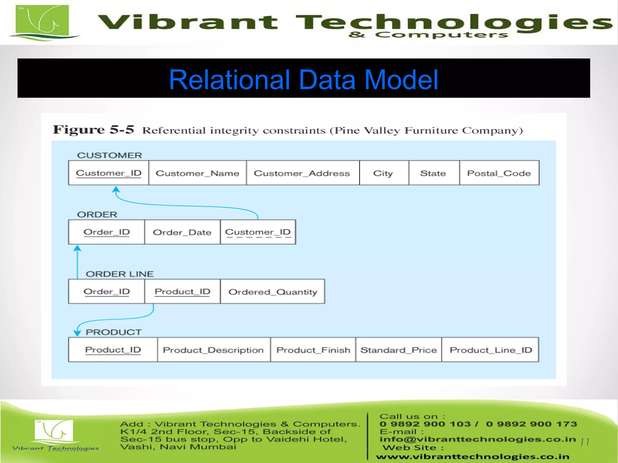
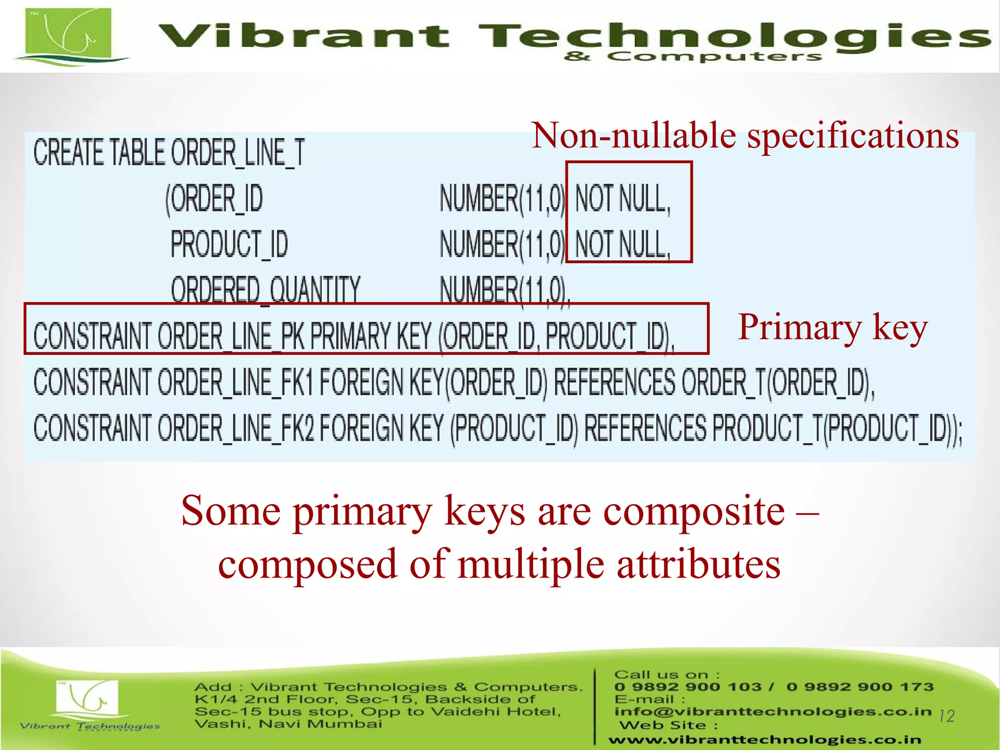
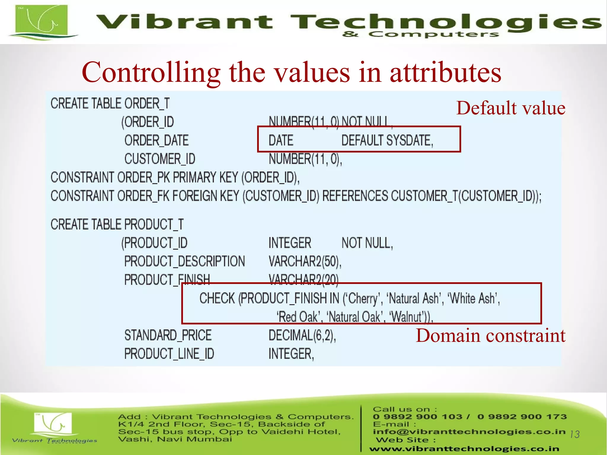
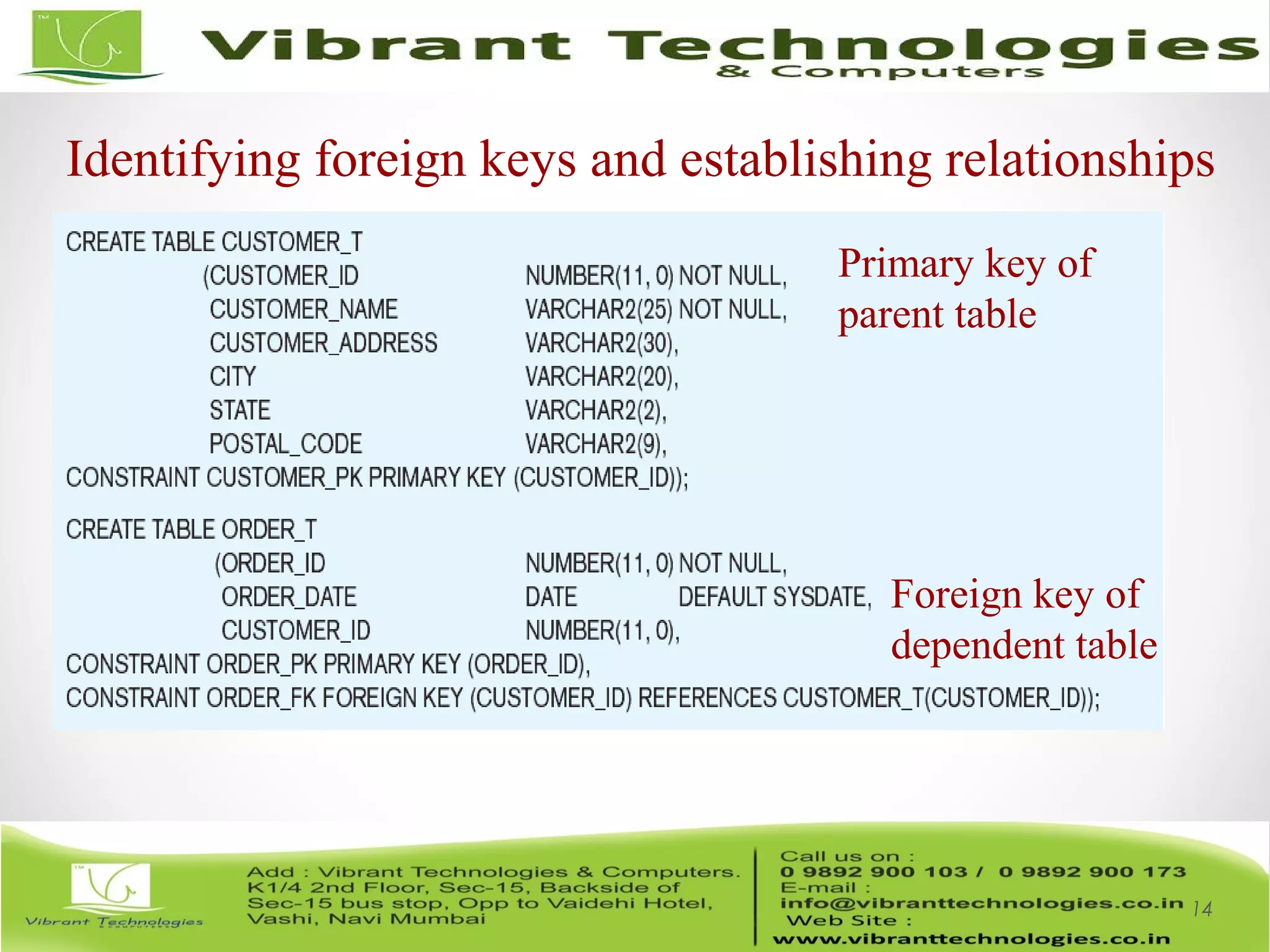
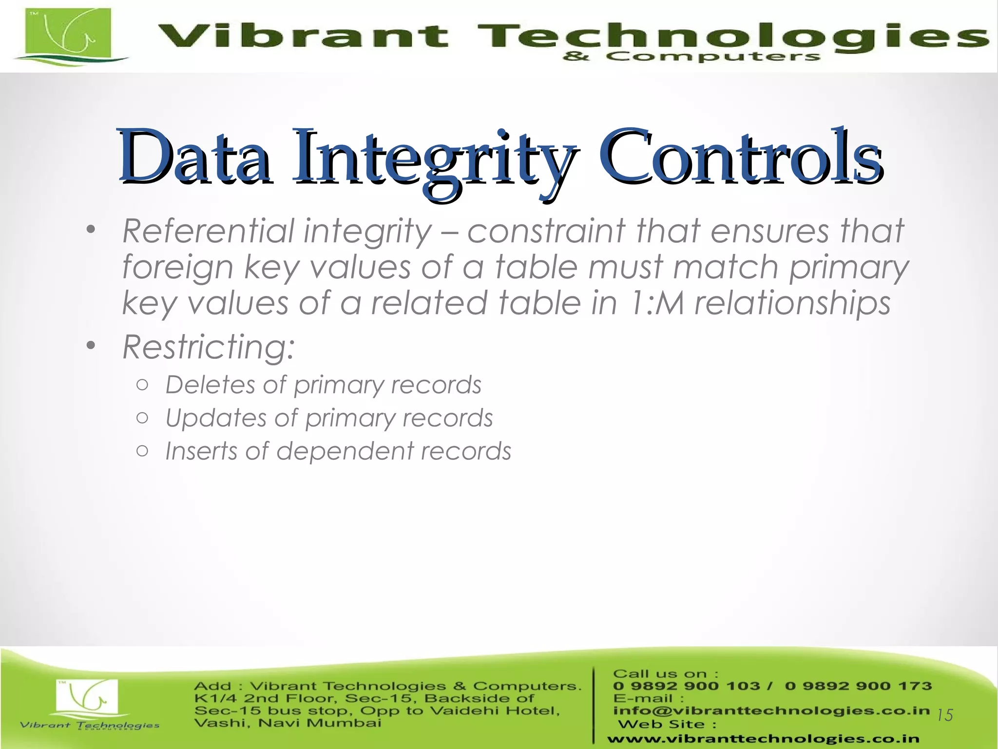
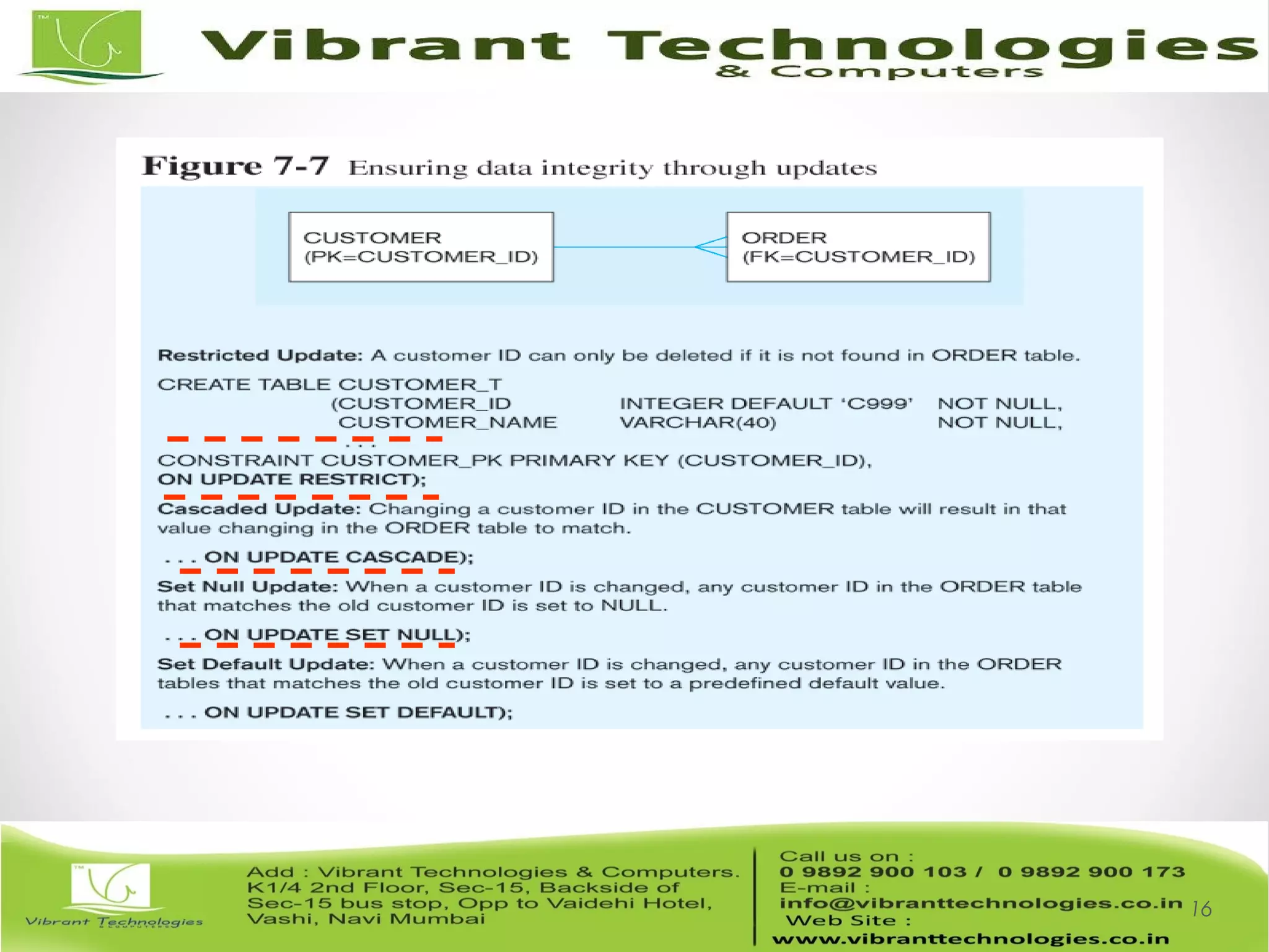

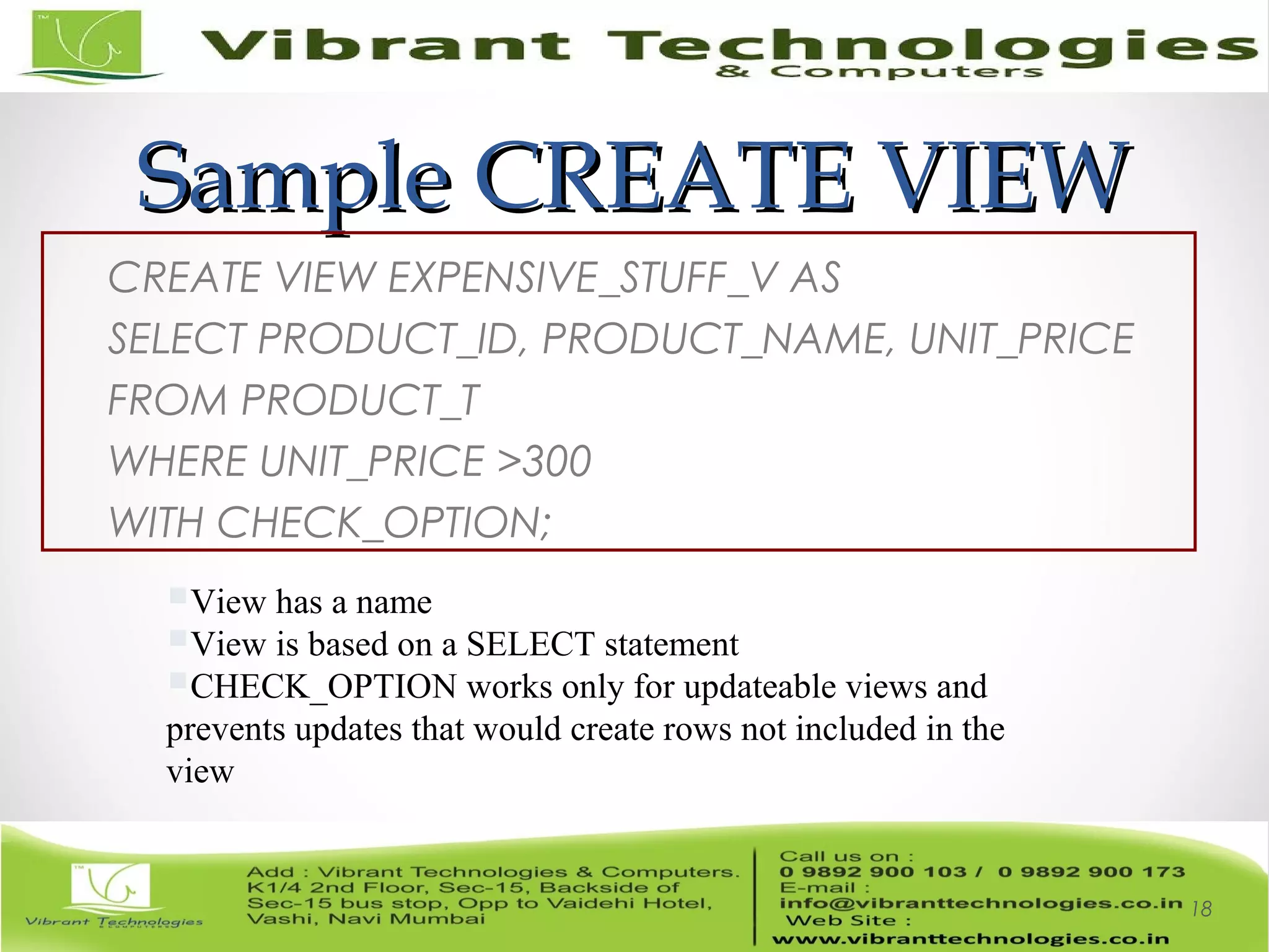
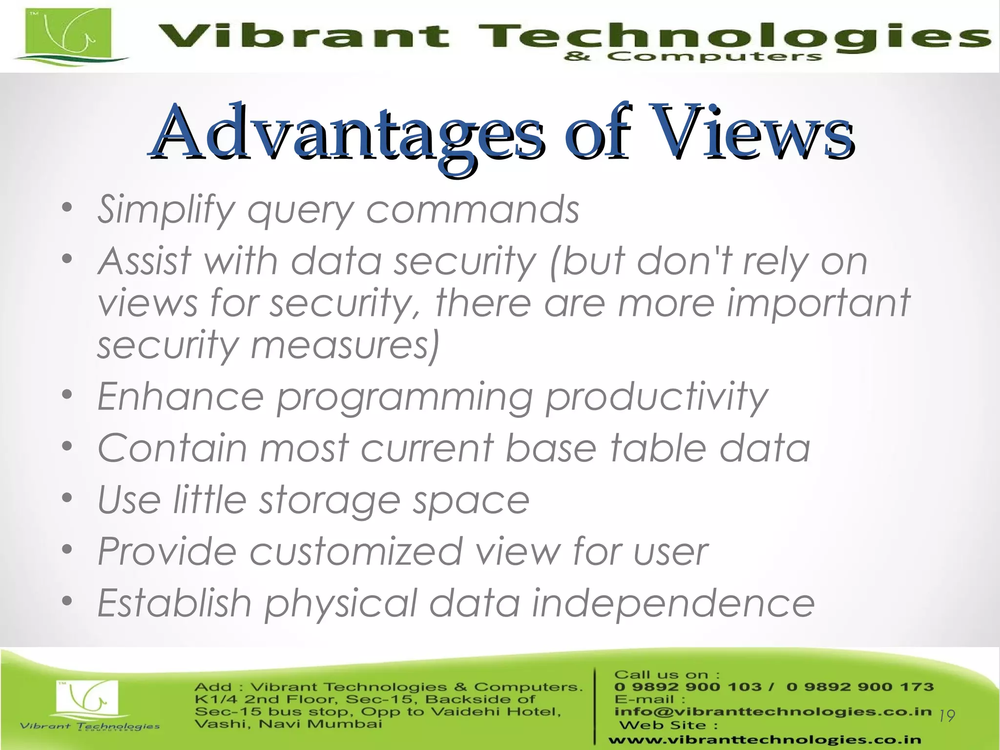

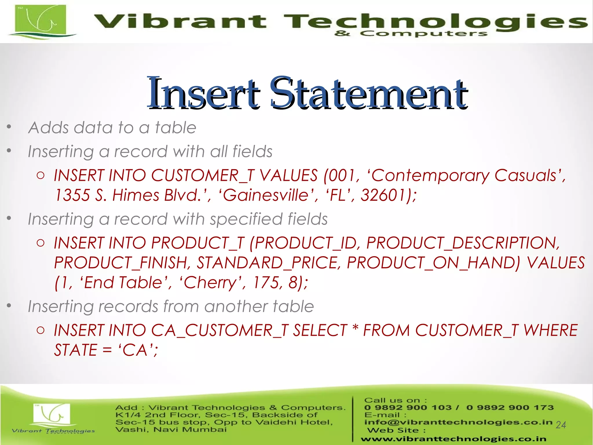
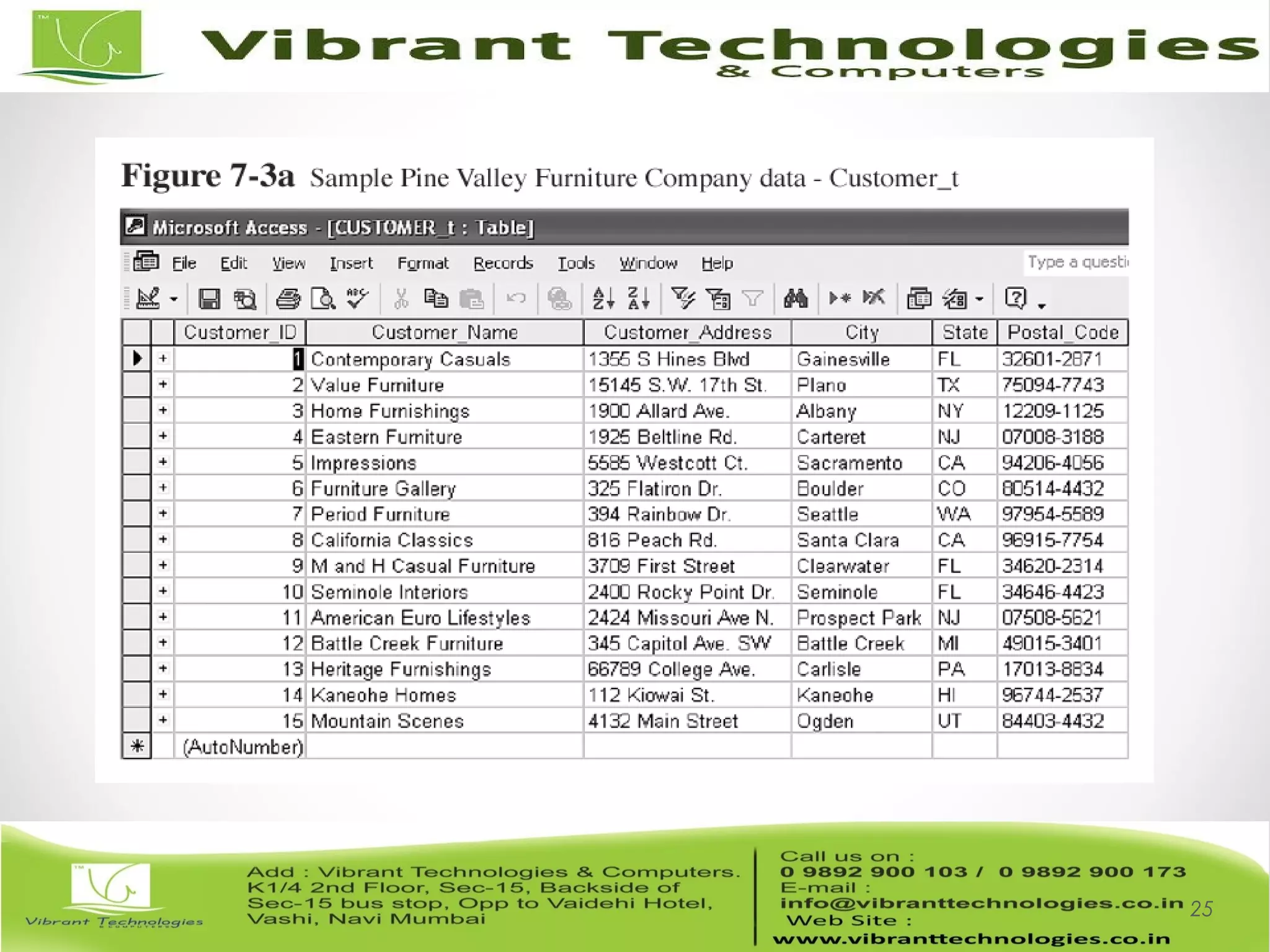
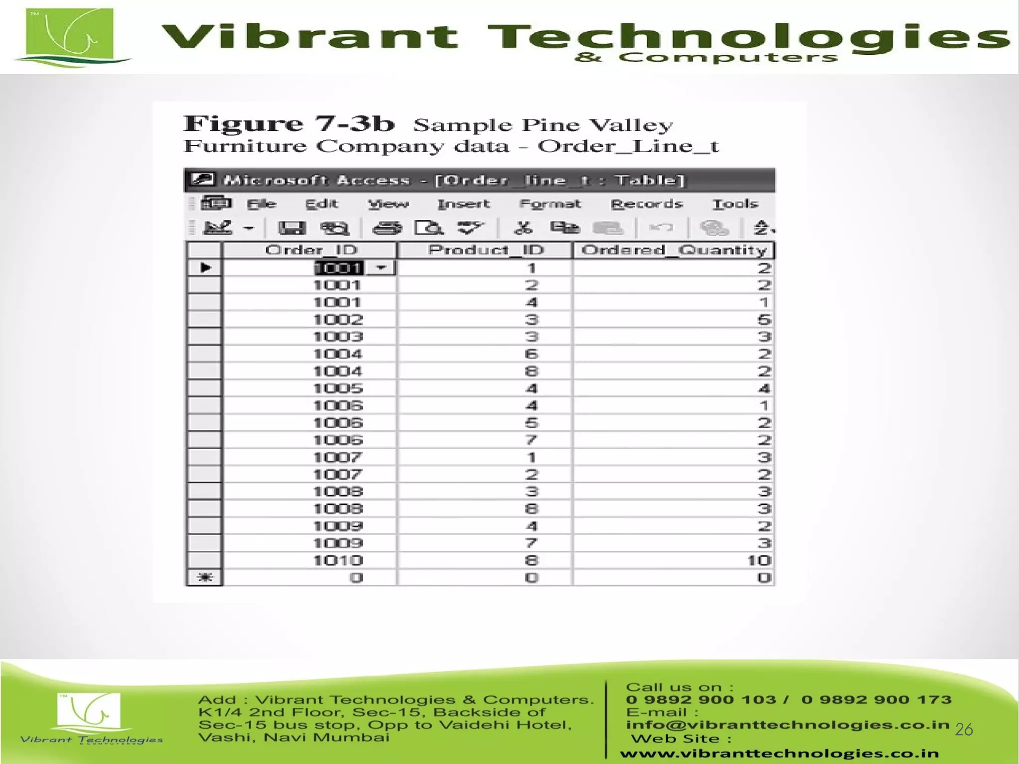
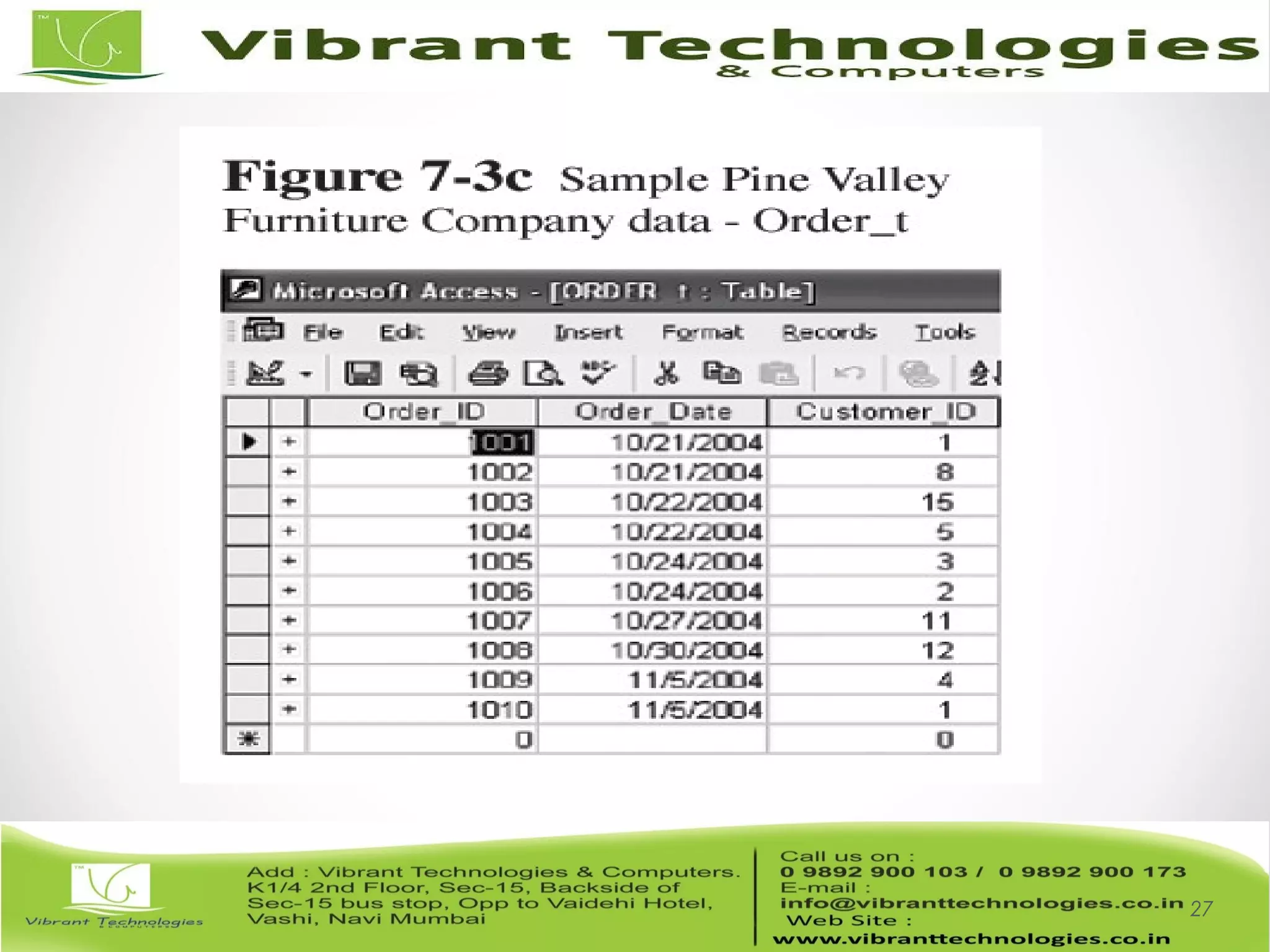
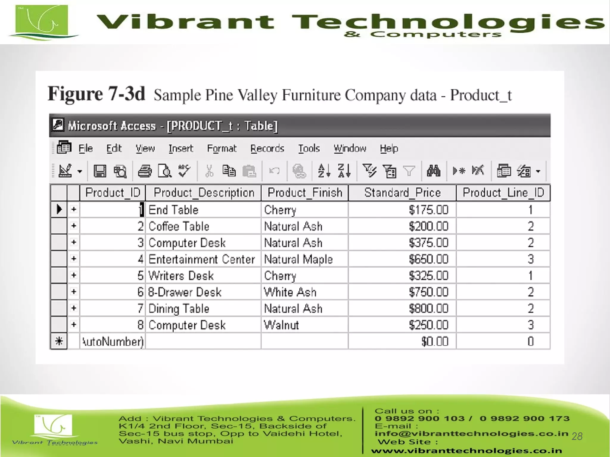
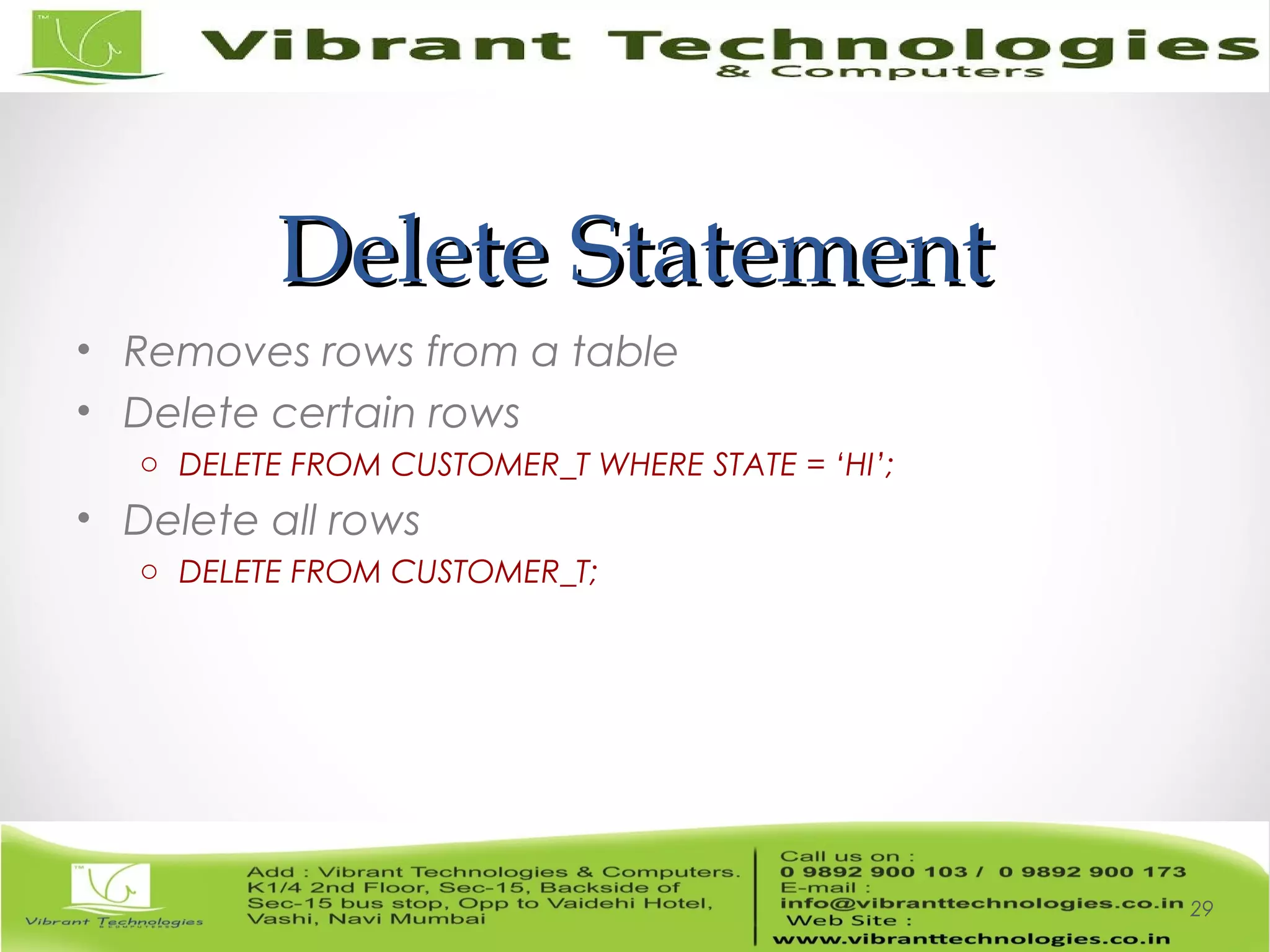
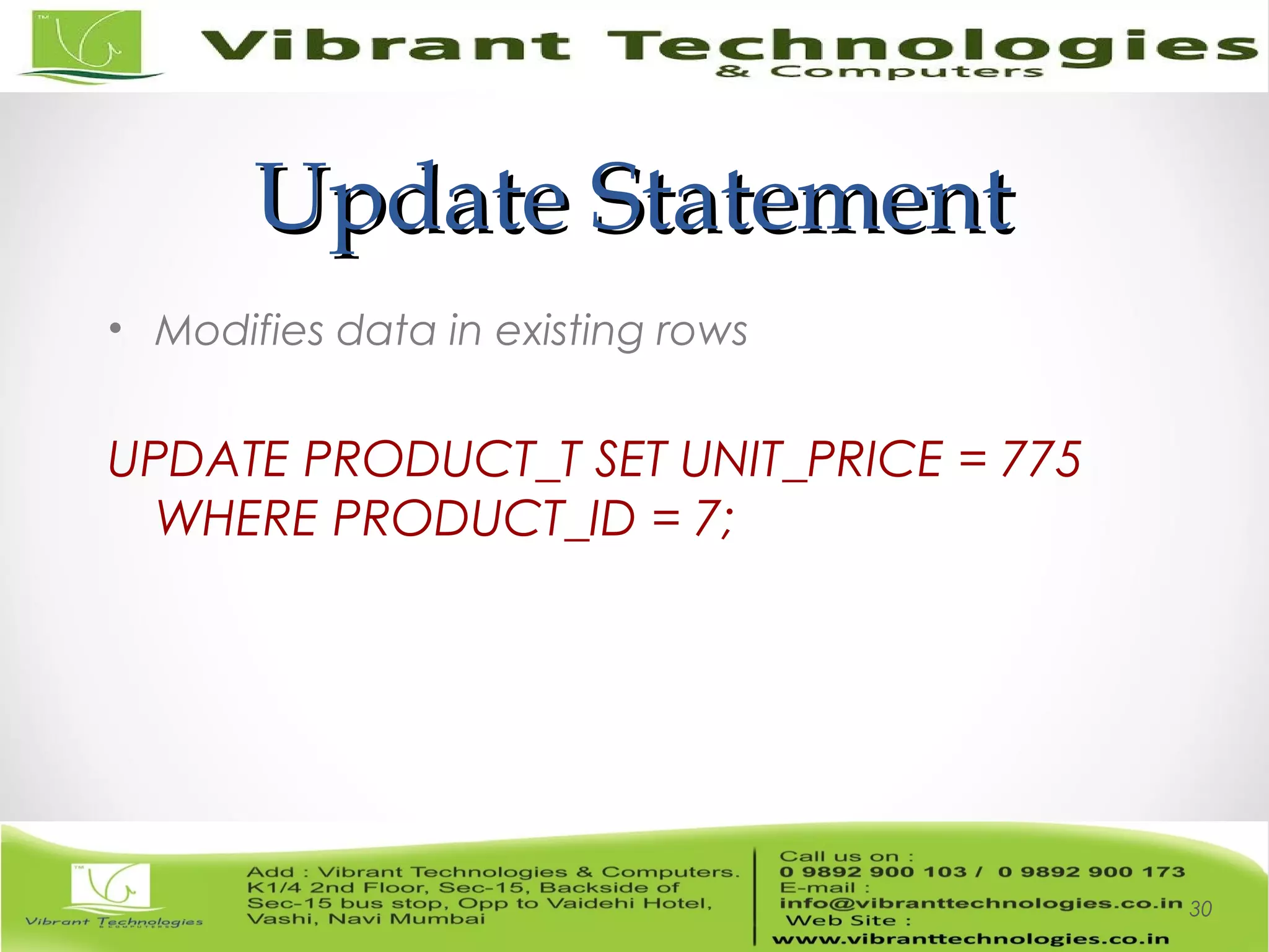
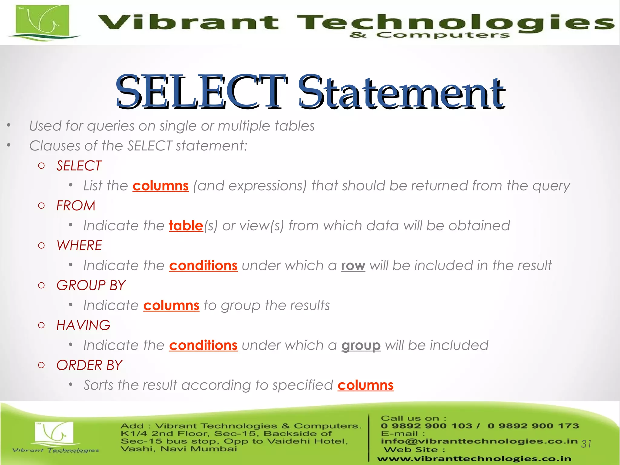
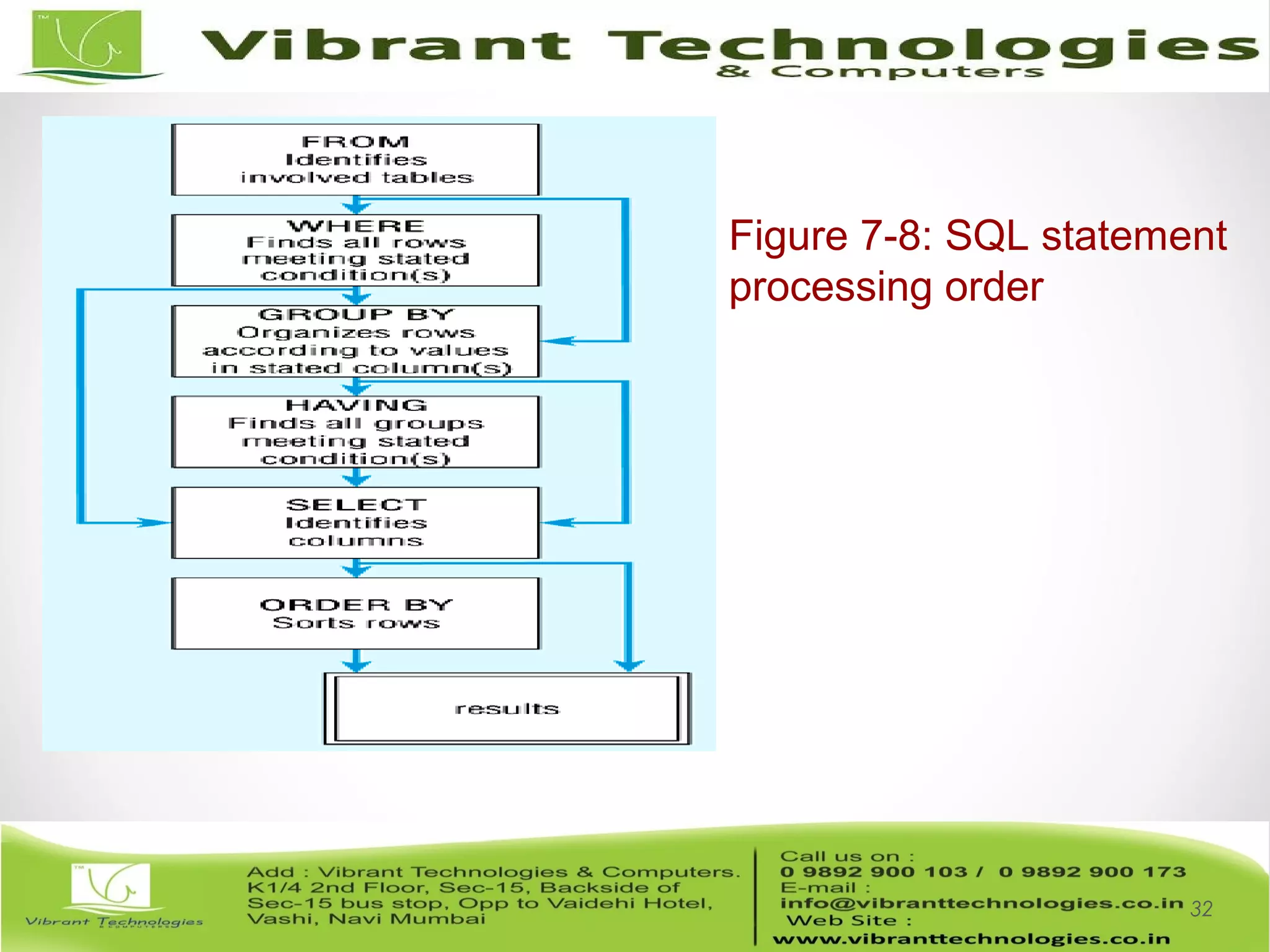
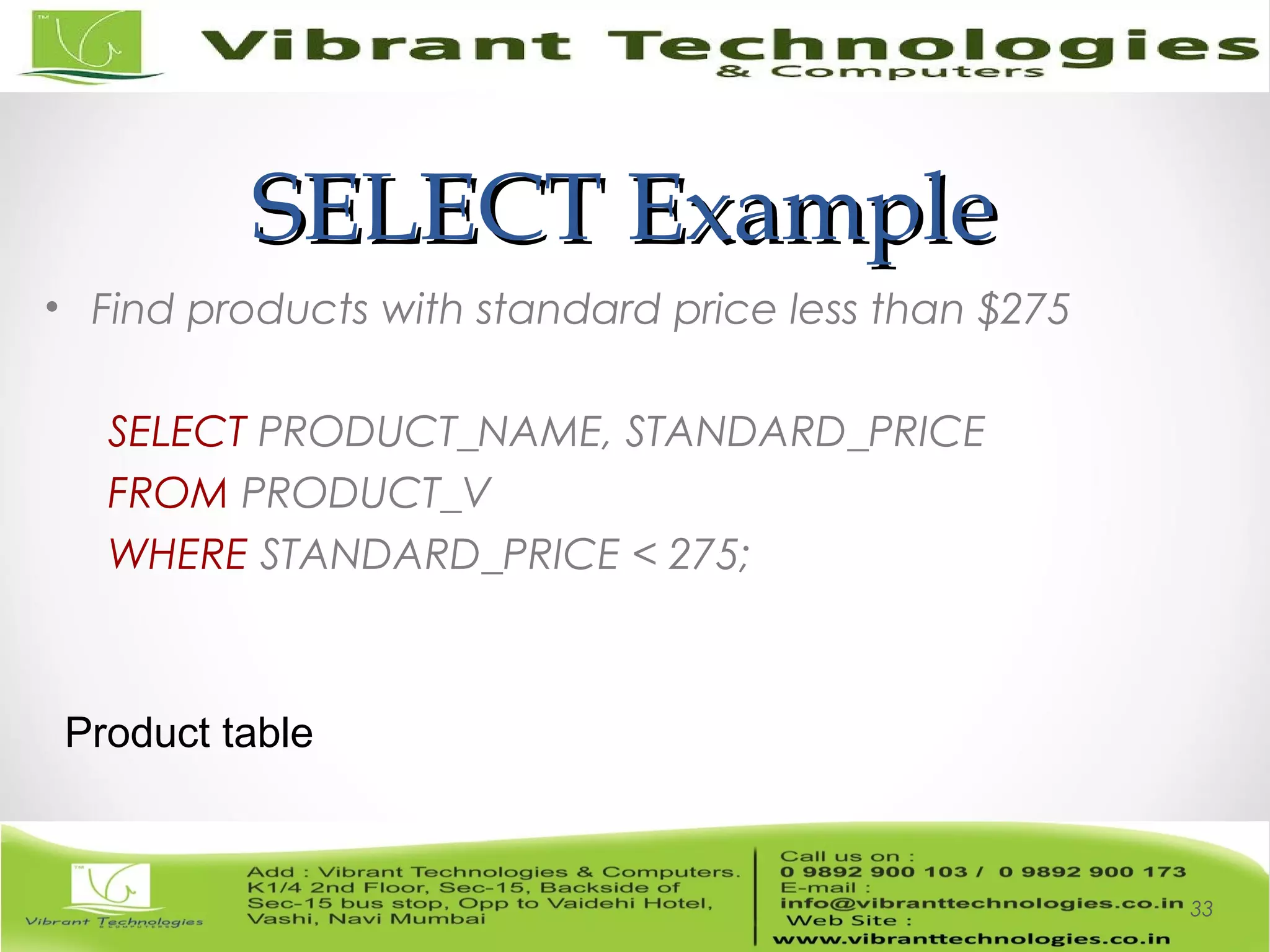
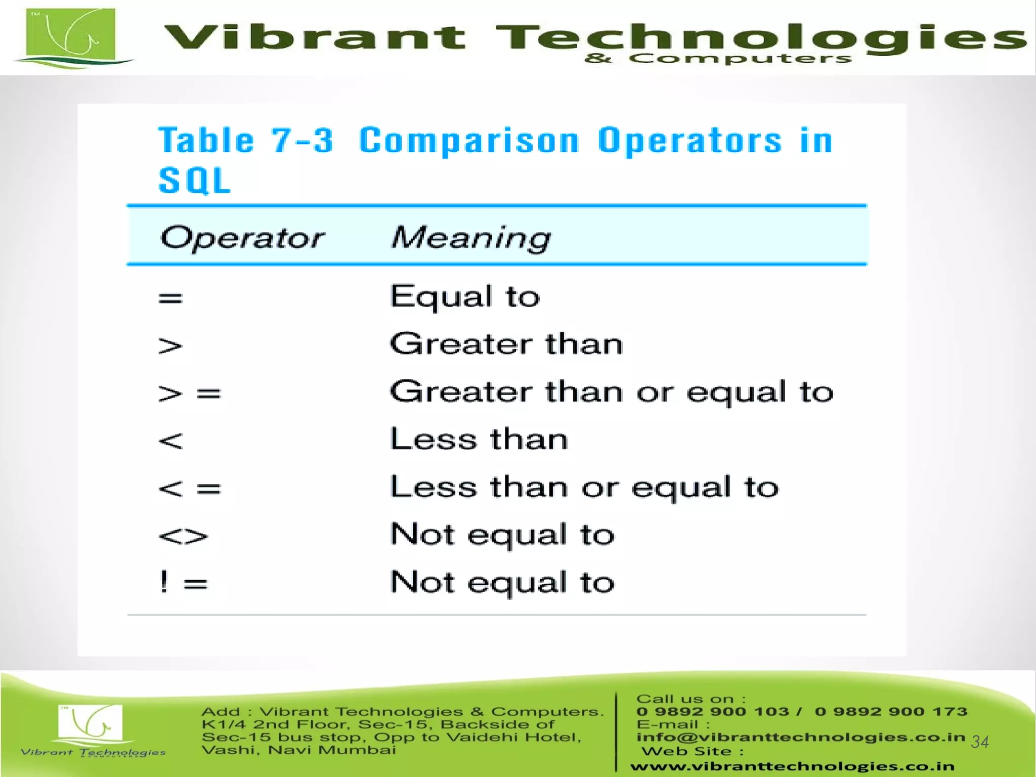
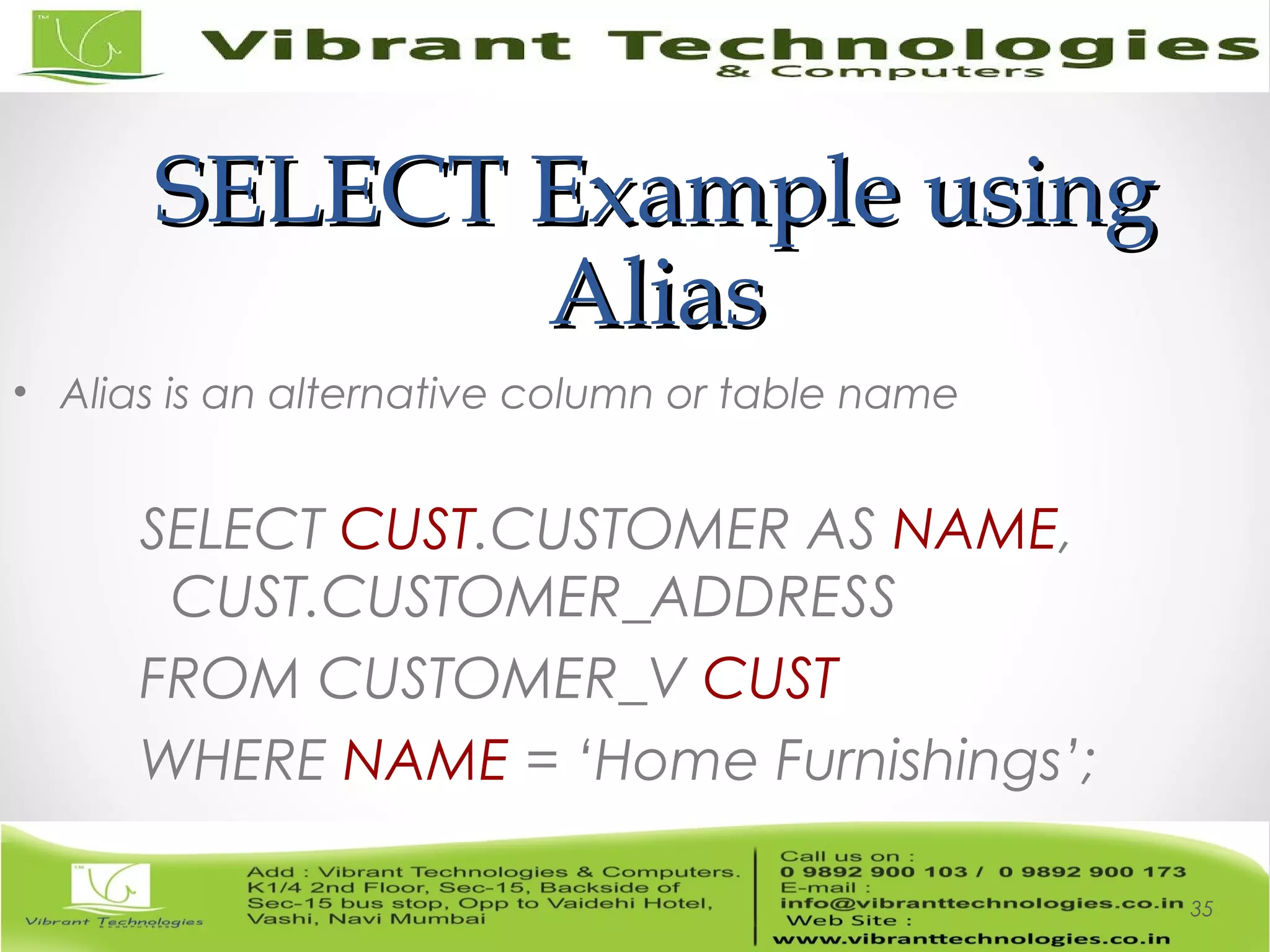
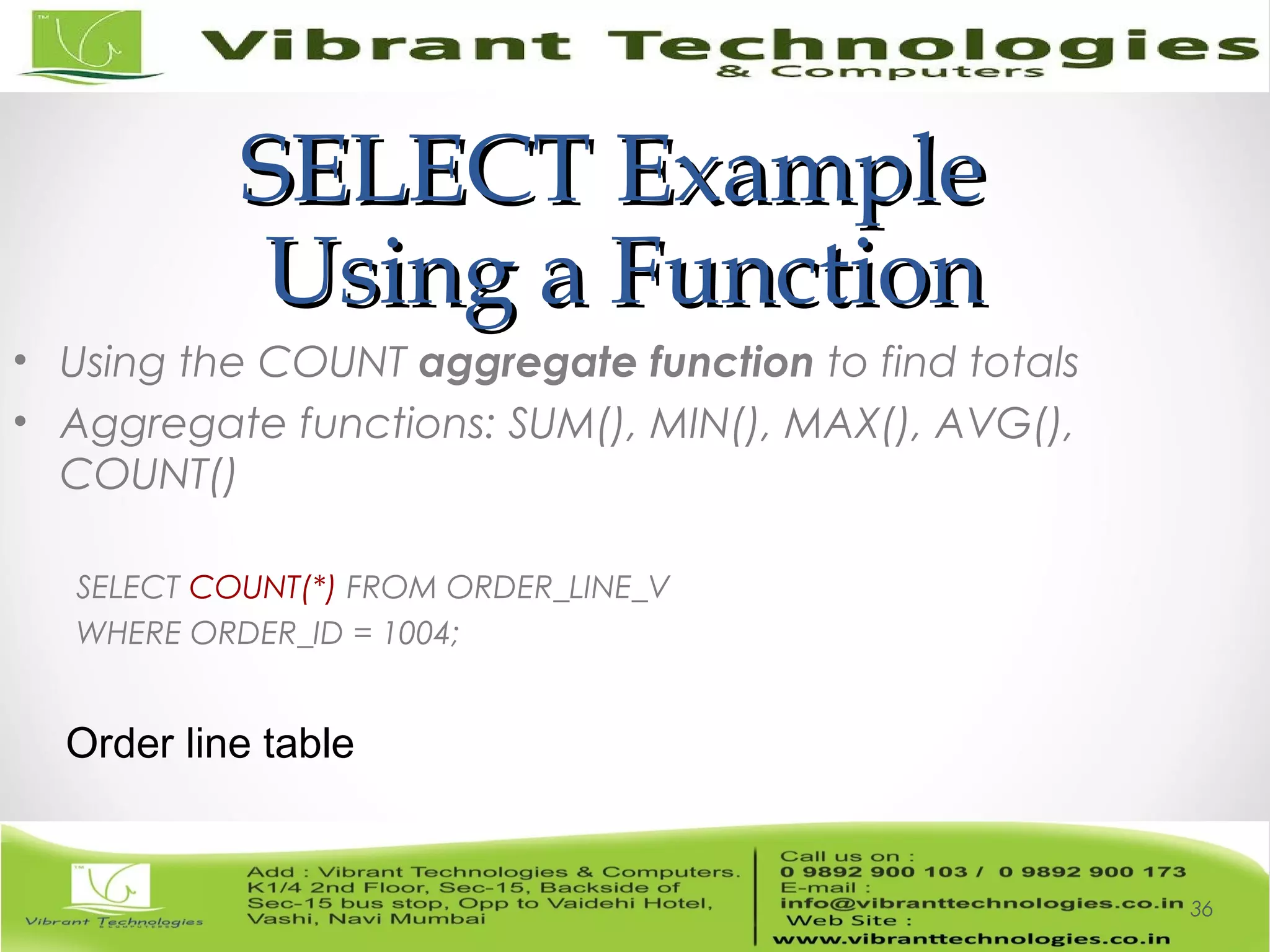
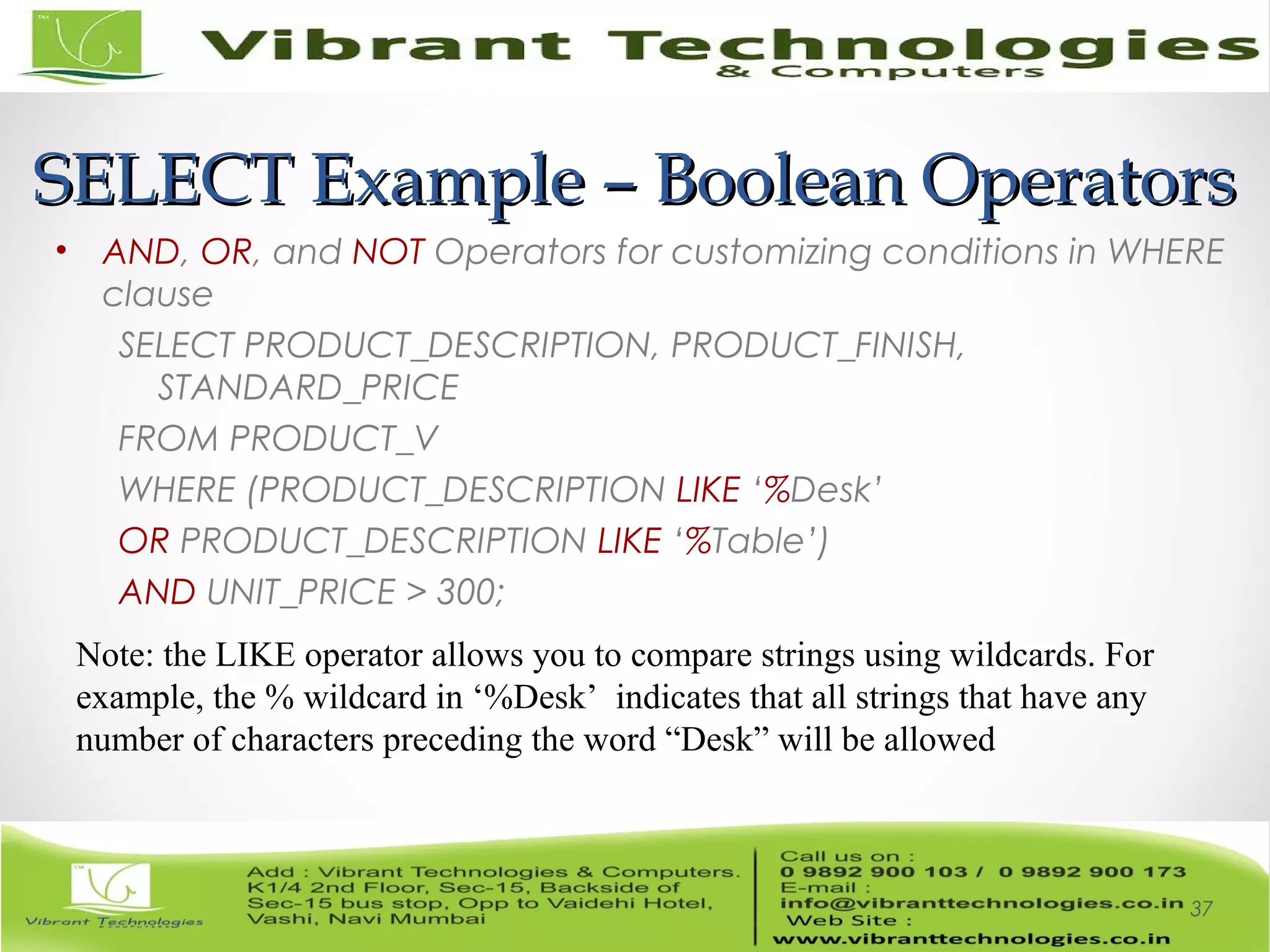
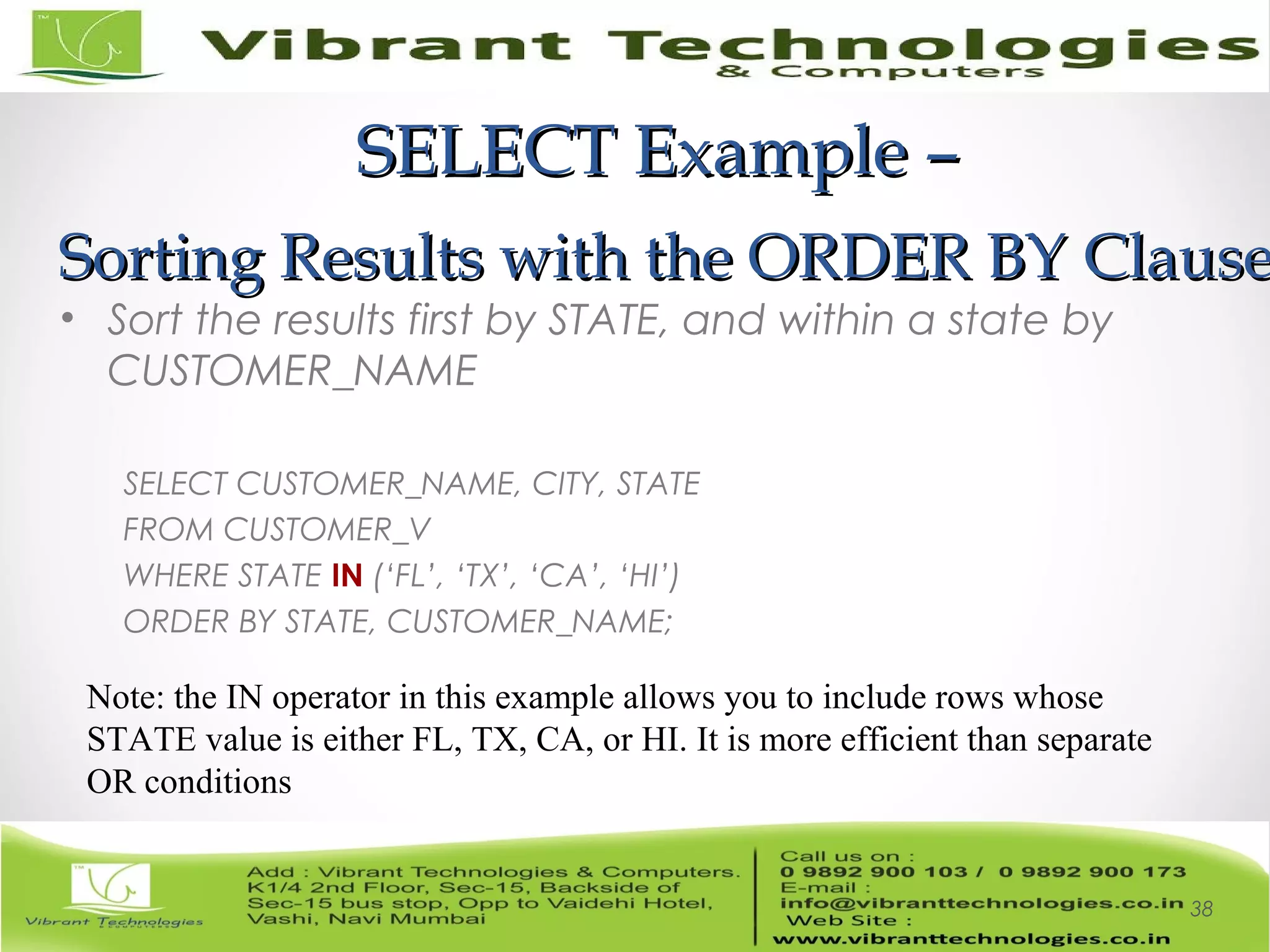
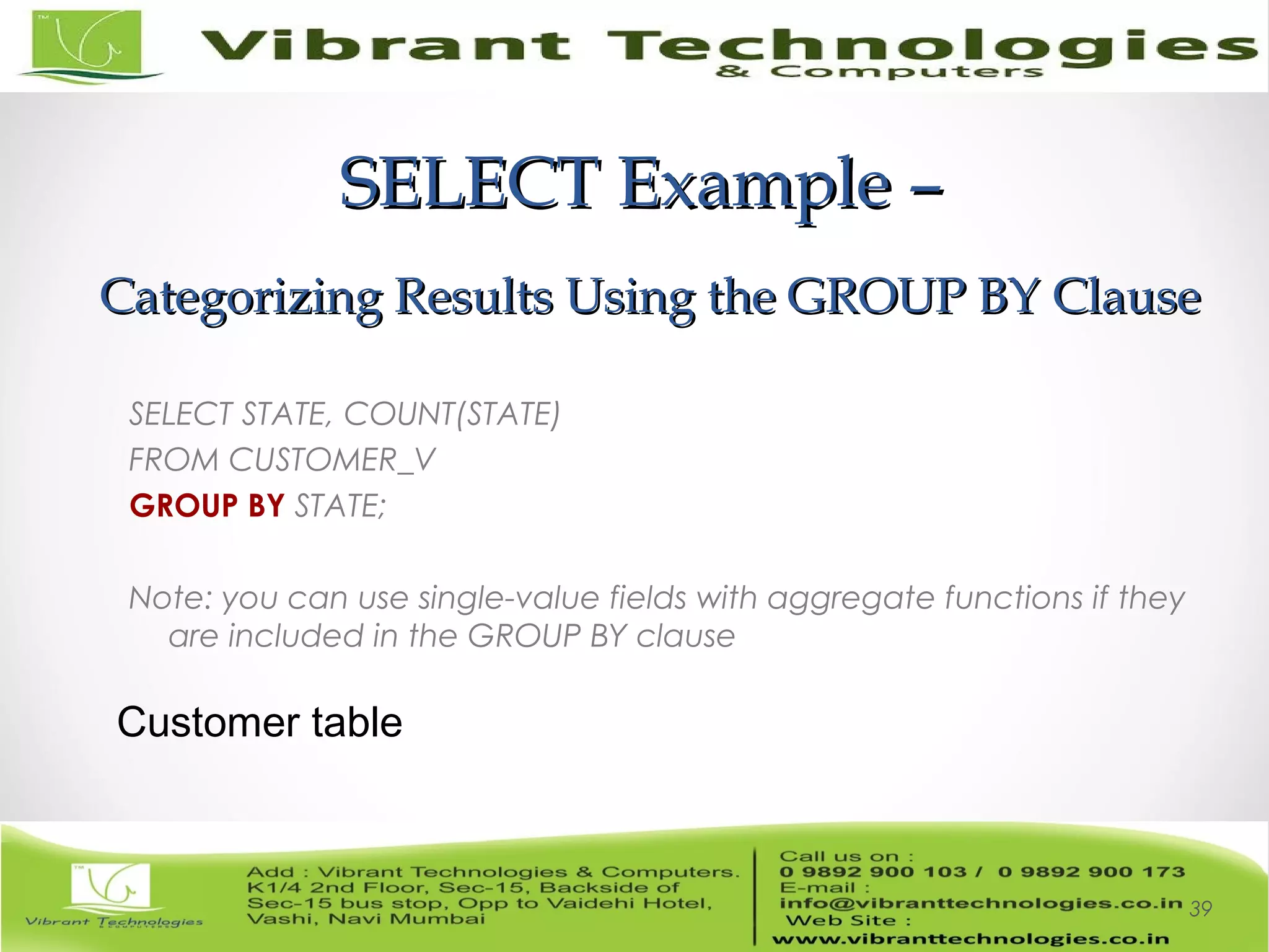
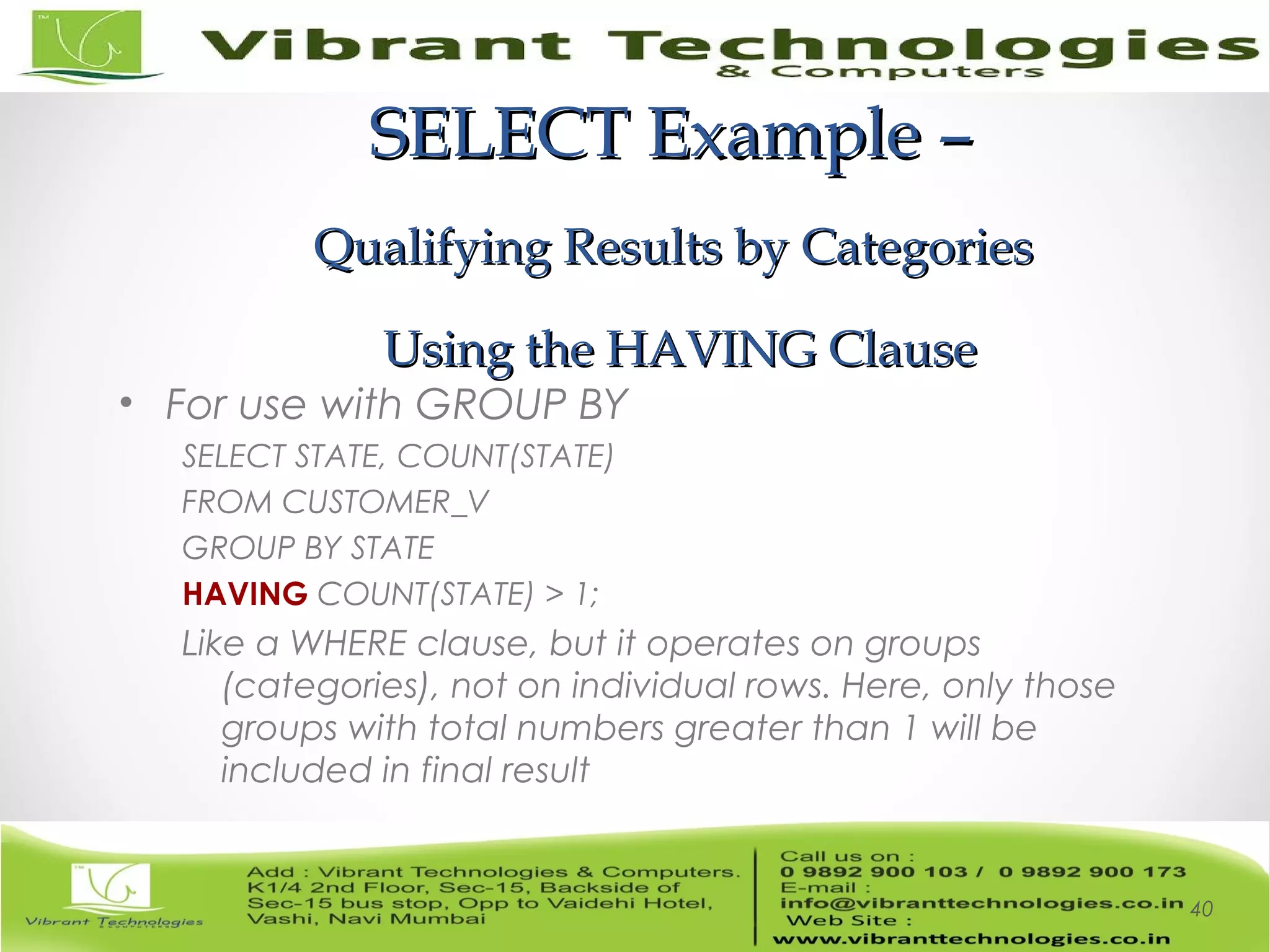


This document provides an introduction to SQL (Structured Query Language) for manipulating and working with data. It covers SQL fundamentals including defining a database using DDL, working with views, writing queries, and establishing referential integrity. It also discusses SQL data types, database definition, creating tables and views, and key SQL statements for data manipulation including SELECT, INSERT, UPDATE, and DELETE. Examples are provided for creating tables and views, inserting, updating, and deleting data, and writing queries using functions, operators, sorting, grouping, and filtering.


![[Www.pkbulk.blogspot.com]dbms10](https://cdn.slidesharecdn.com/ss_thumbnails/www-pkbul-blogspot-comdbms10-130615034621-phpapp01-thumbnail.jpg?width=600ounds&width=560&fit=bounds)


![UiPath Automation Suite Installation (Hands-On) [2/3]](https://cdn.slidesharecdn.com/ss_thumbnails/automationsuitecommunitysession2-251015095633-a6d862f1-thumbnail.jpg?width=600ounds&width=560&fit=bounds)


