Download to read offline
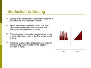

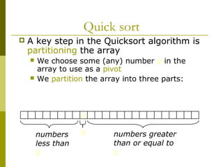
![Quick sort
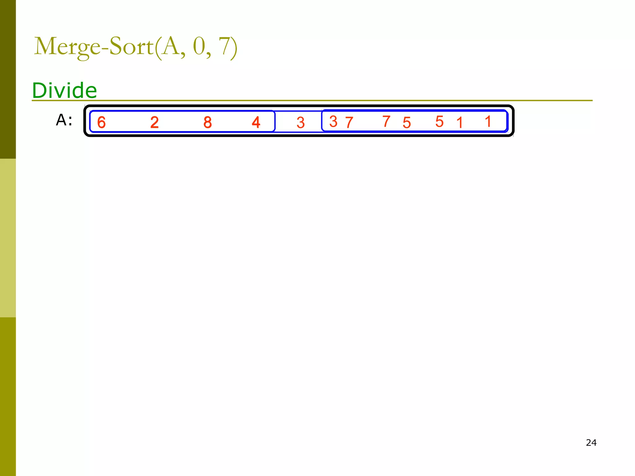
To sort a[left...right]:
1. if left < right:
1.1. Partition a[left...right] such that:
all a[left...p-1] are less than a[p], and
all a[p+1...right] are >= a[p]
1.2. Quicksort a[left...p-1]
1.3. Quicksort a[p+1...right]
2. Terminate](https://image.slidesharecdn.com/sorting-180808153102/85/Sorting-9-320.jpg)
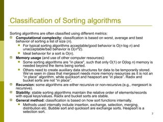
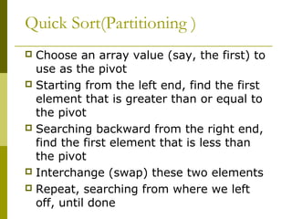
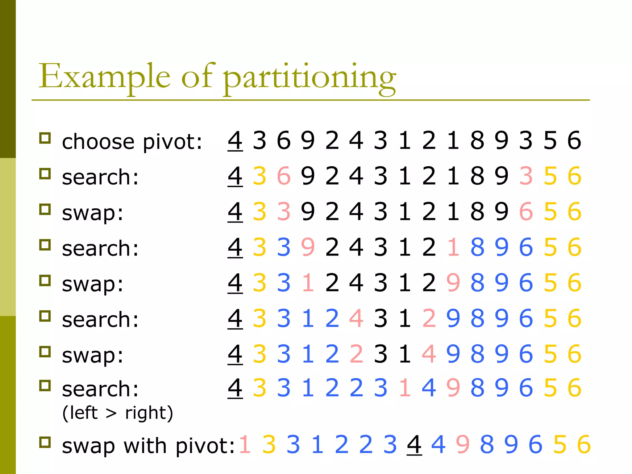
![Partitioning
To partition a[left...right]:
1. Set p = a[left], l = left + 1, r = right;
2. while l < r, do
2.1. while l < right && a[l] < p { l = l + 1 }
2.2. while r > left && a[r] >= p { r = r – 1}
2.3. if l < r { swap a[l] and a[r] }
3. a[left] = a[r]; a[r] = p;
4. Terminate](https://image.slidesharecdn.com/sorting-180808153102/85/Sorting-10-320.jpg)

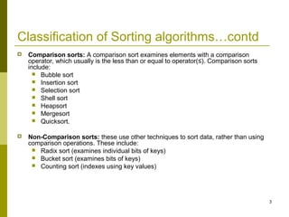
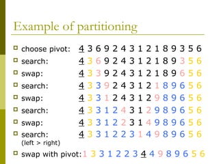
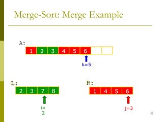
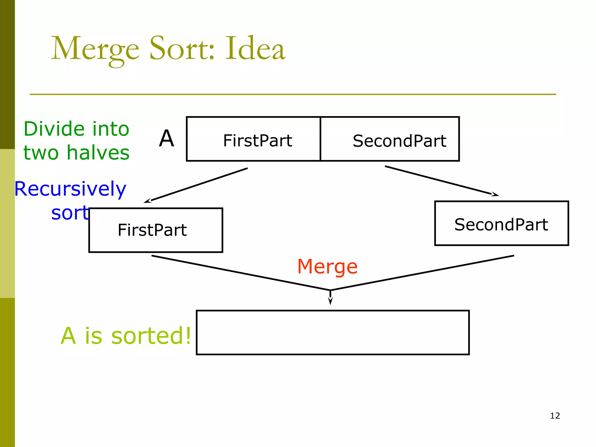
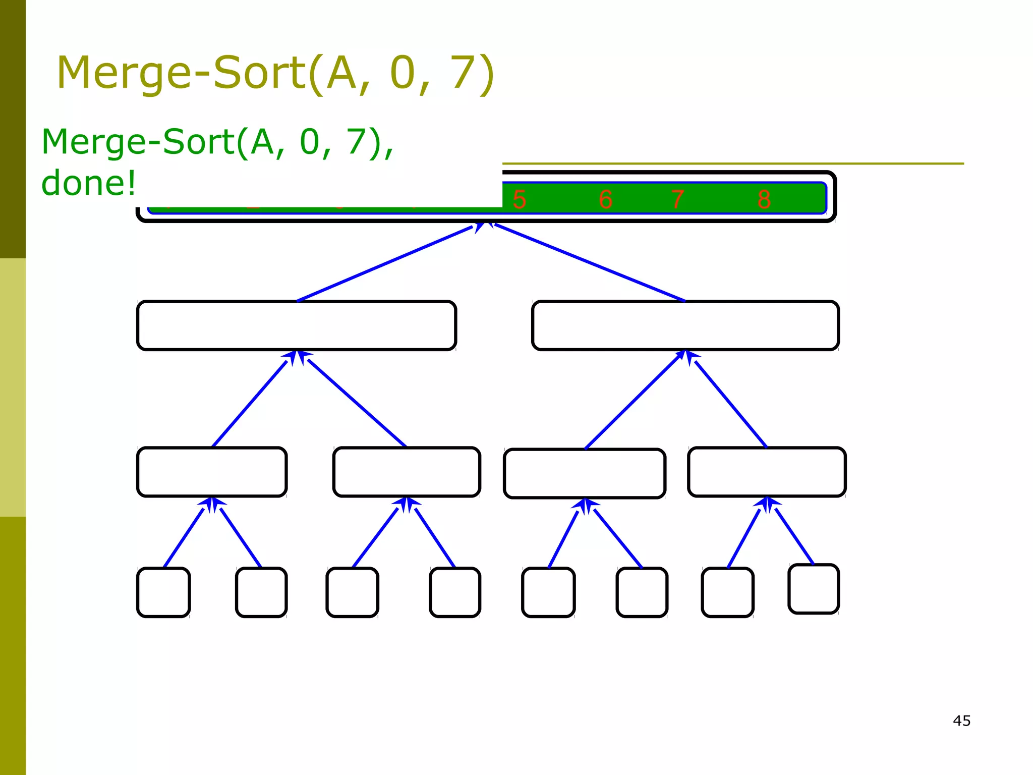
![13
A[middle]A[middle]A[left]A[left]
SortedSorted
FirstPartFirstPart
SortedSorted
SecondPartSecondPart
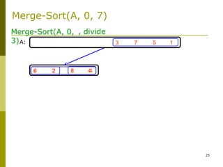
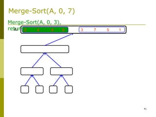
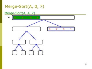
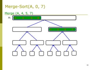
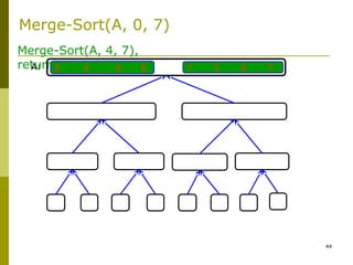
Merge-Sort: Merge
A[right]A[right]
mergemerge
A:A:
A:A:
SortedSorted](https://image.slidesharecdn.com/sorting-180808153102/85/Sorting-13-320.jpg)
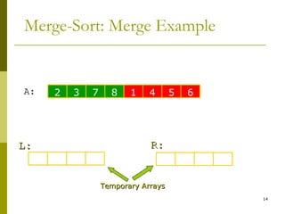

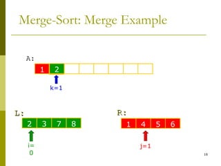
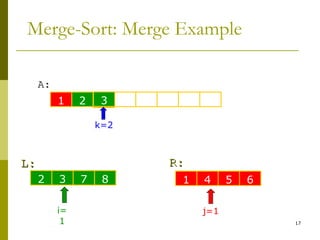

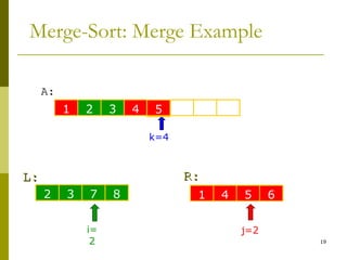
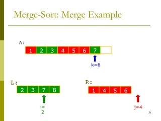

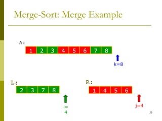
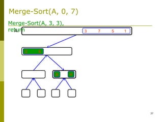
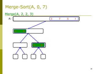
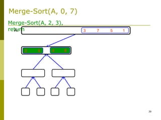
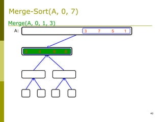
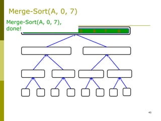
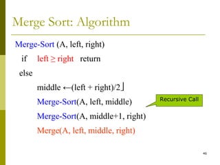
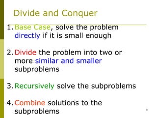
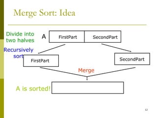
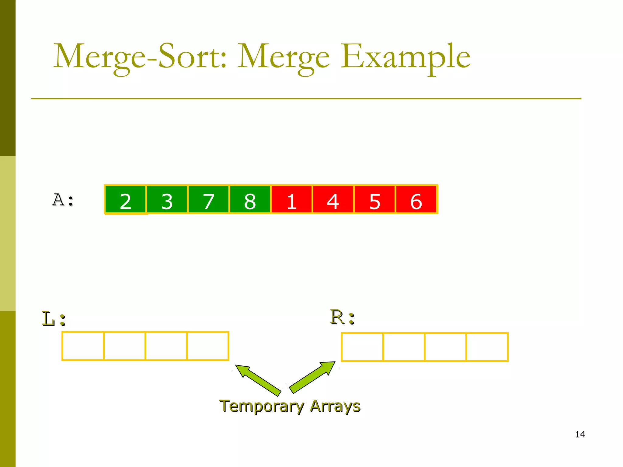
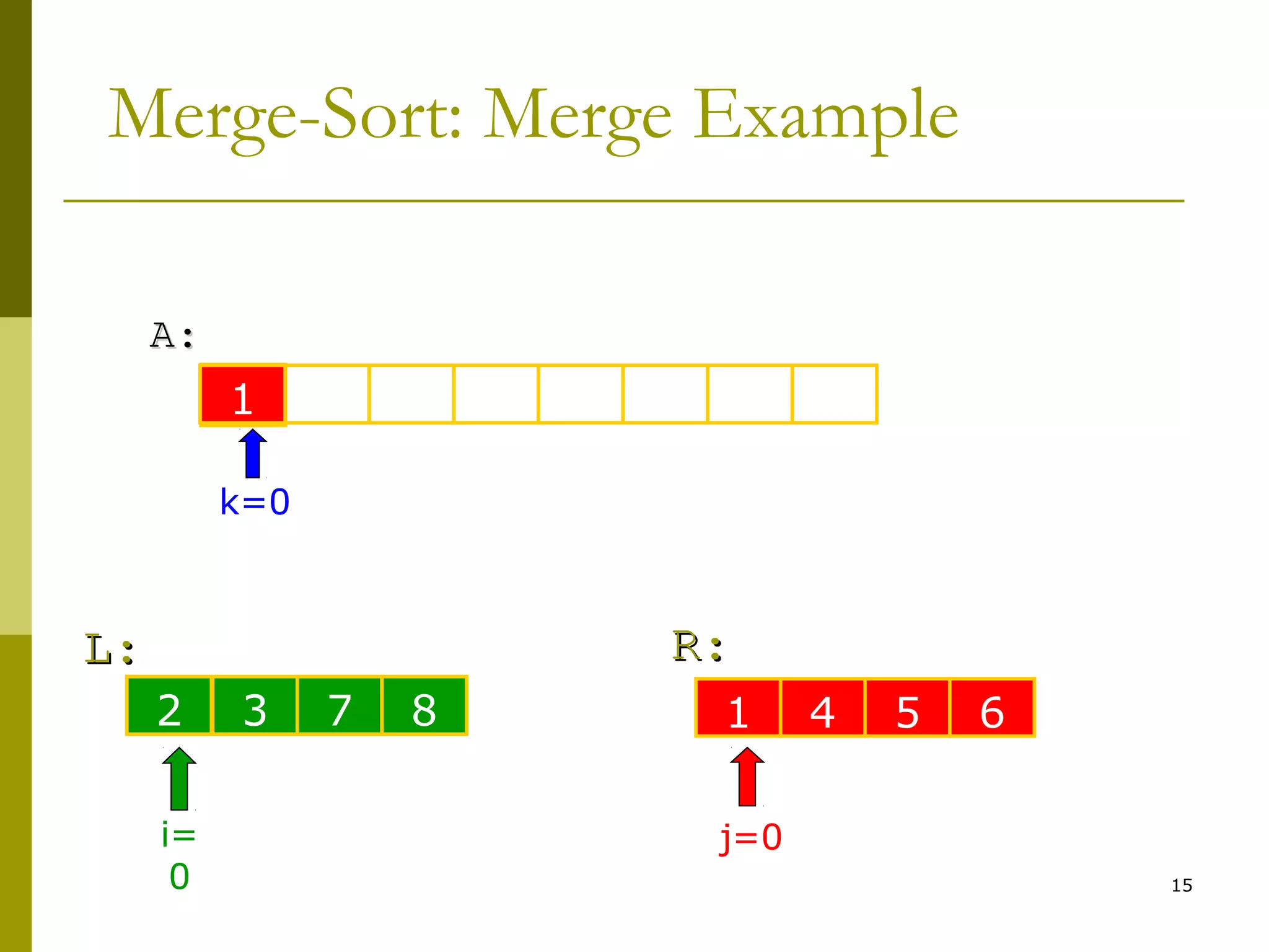
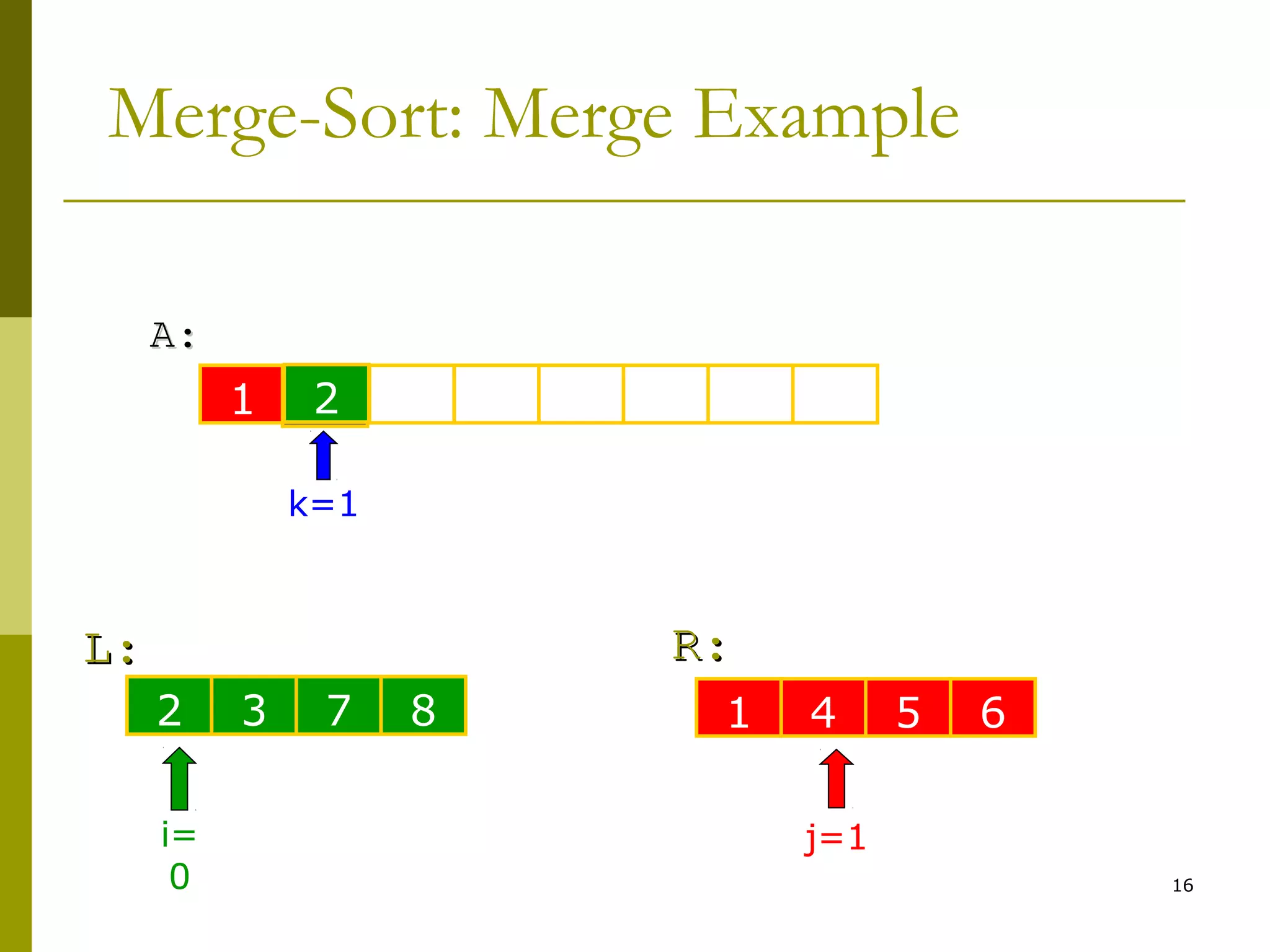
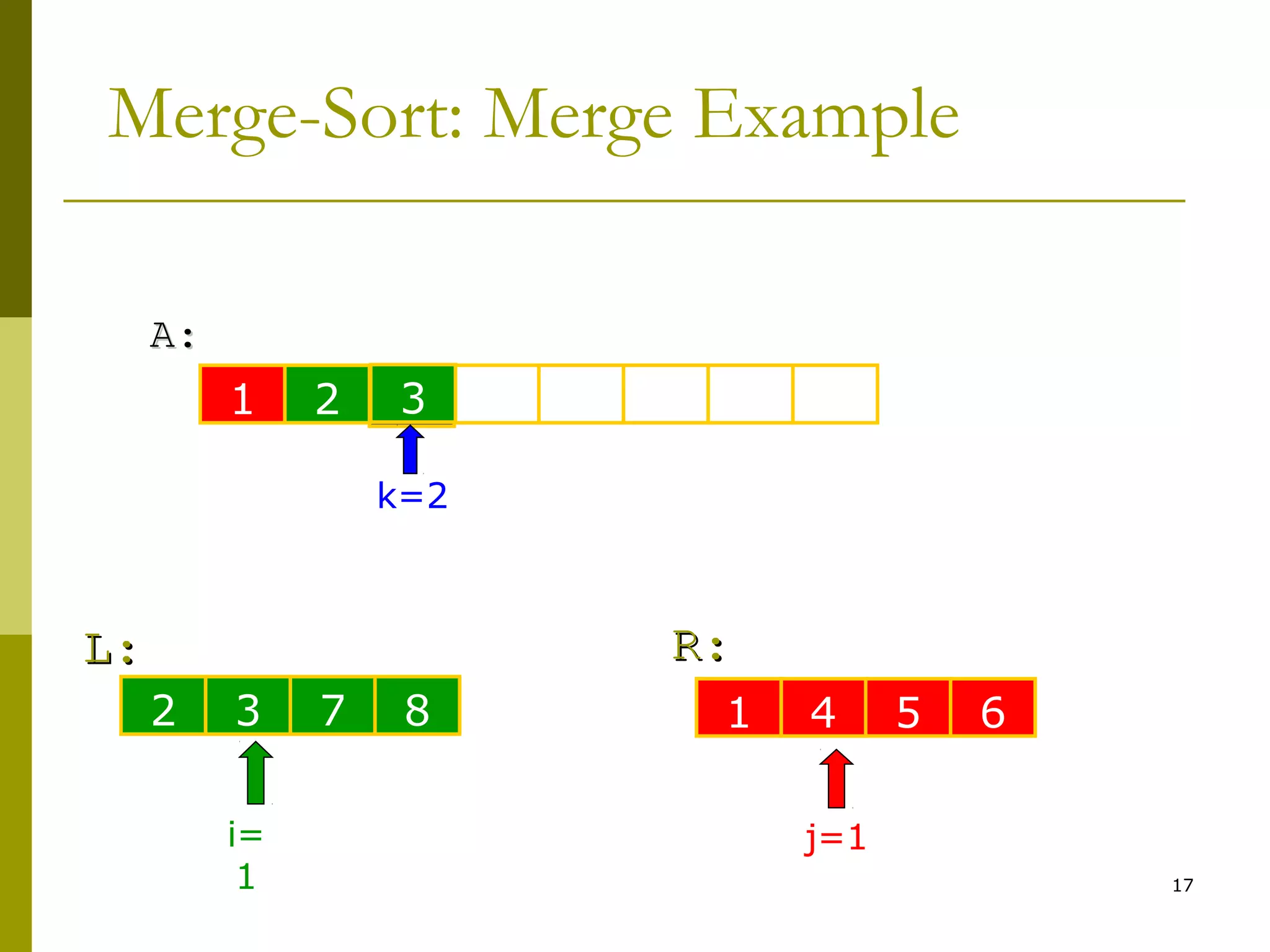
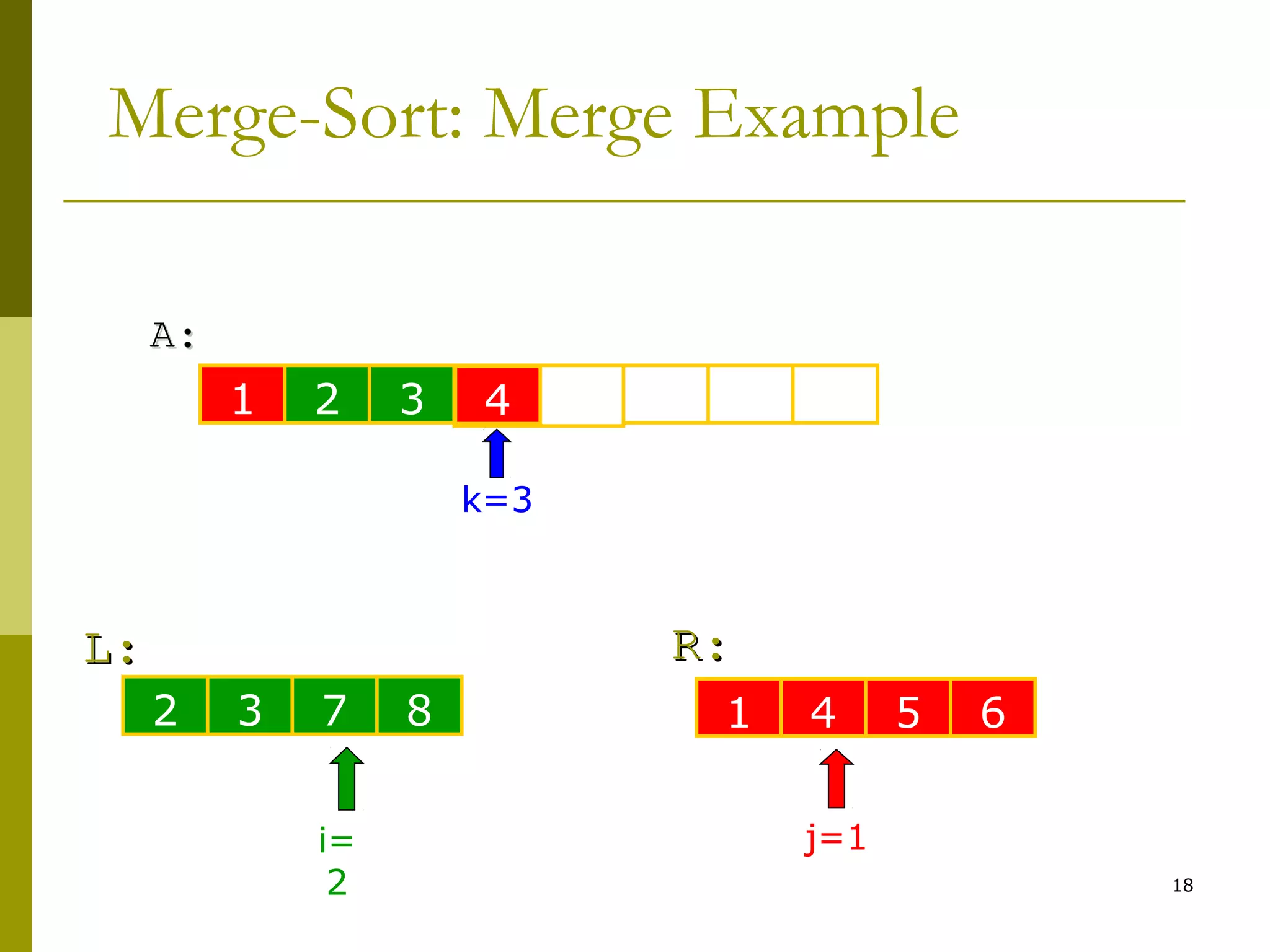
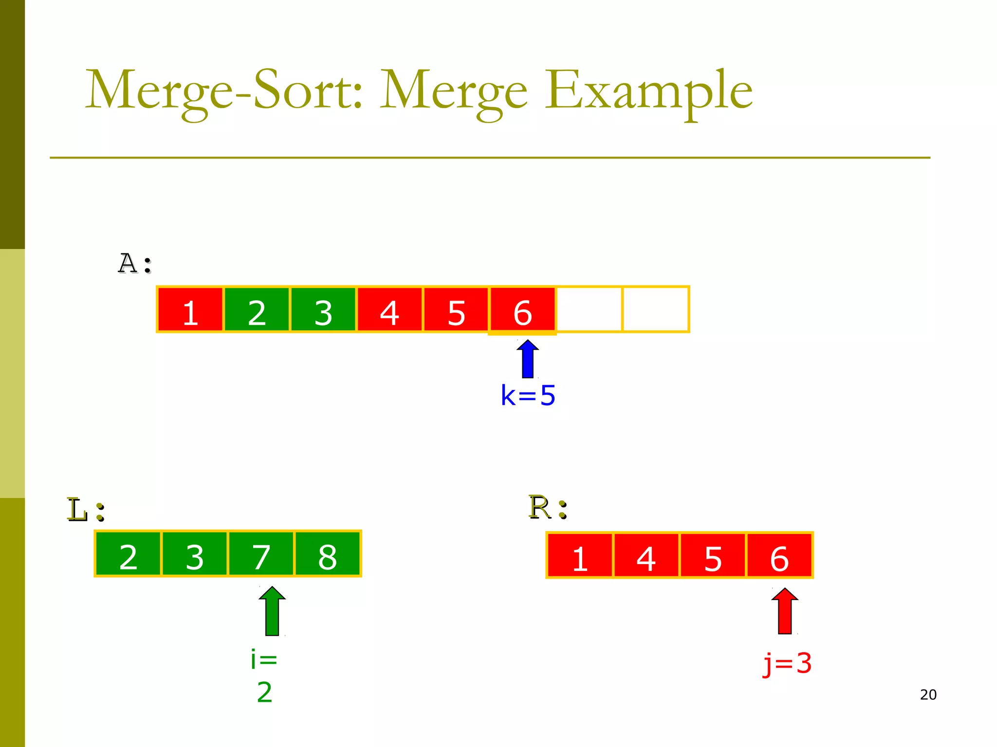
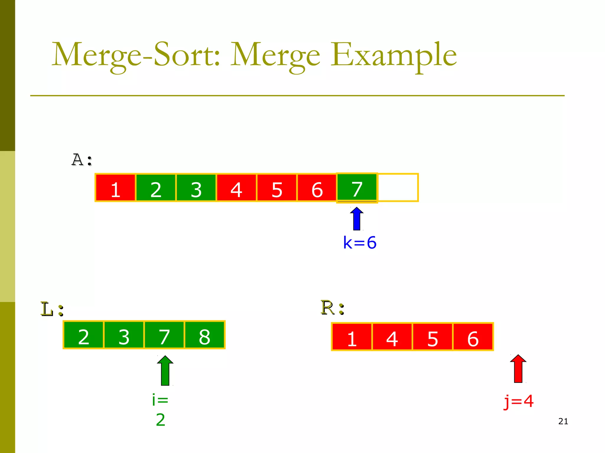
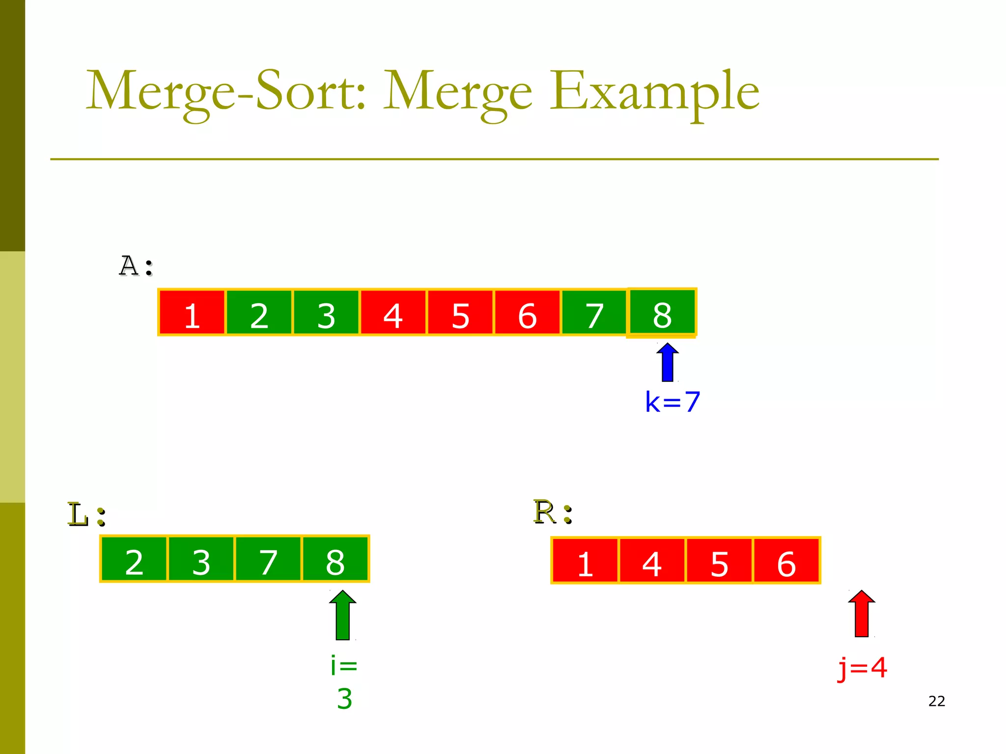
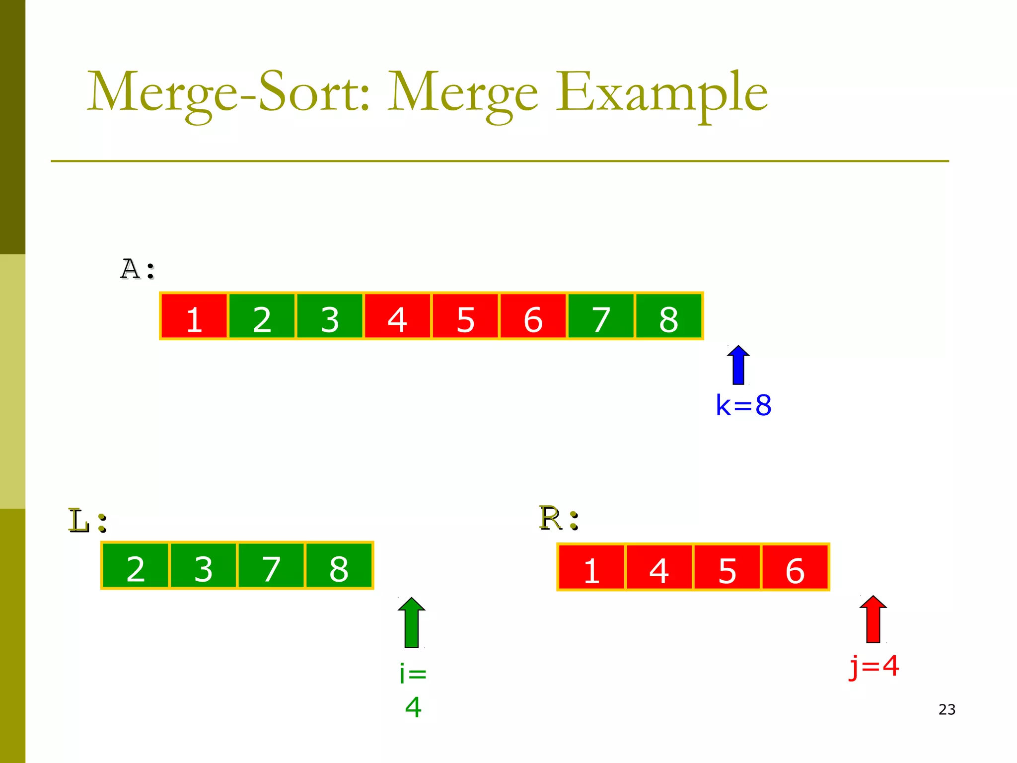
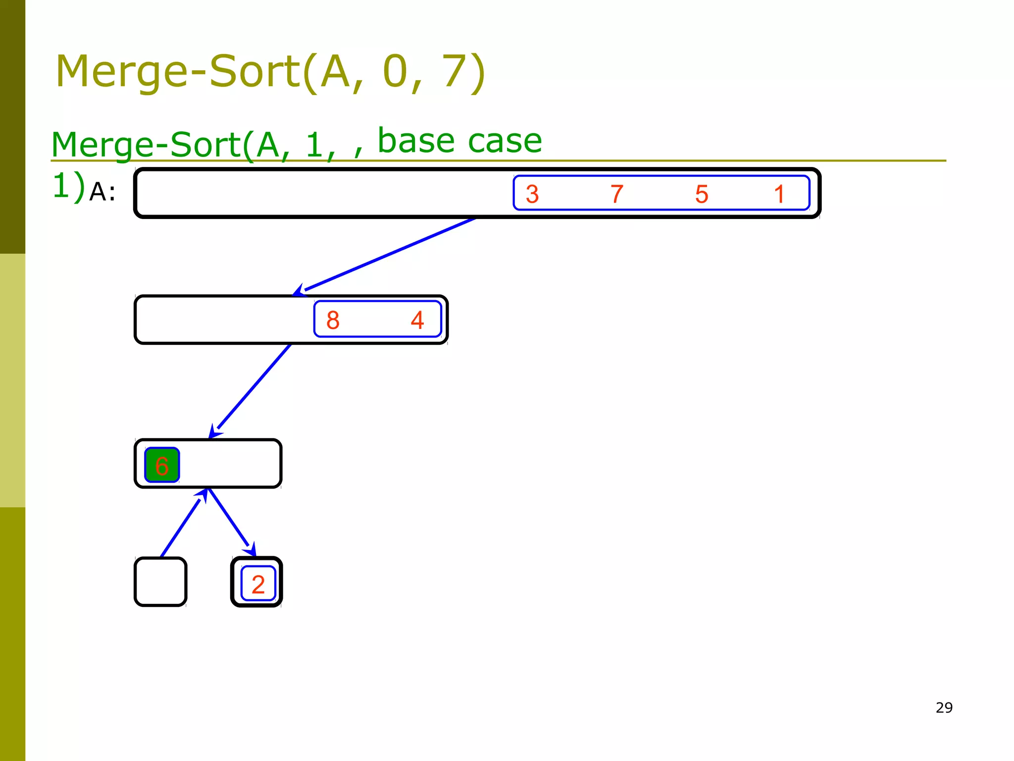
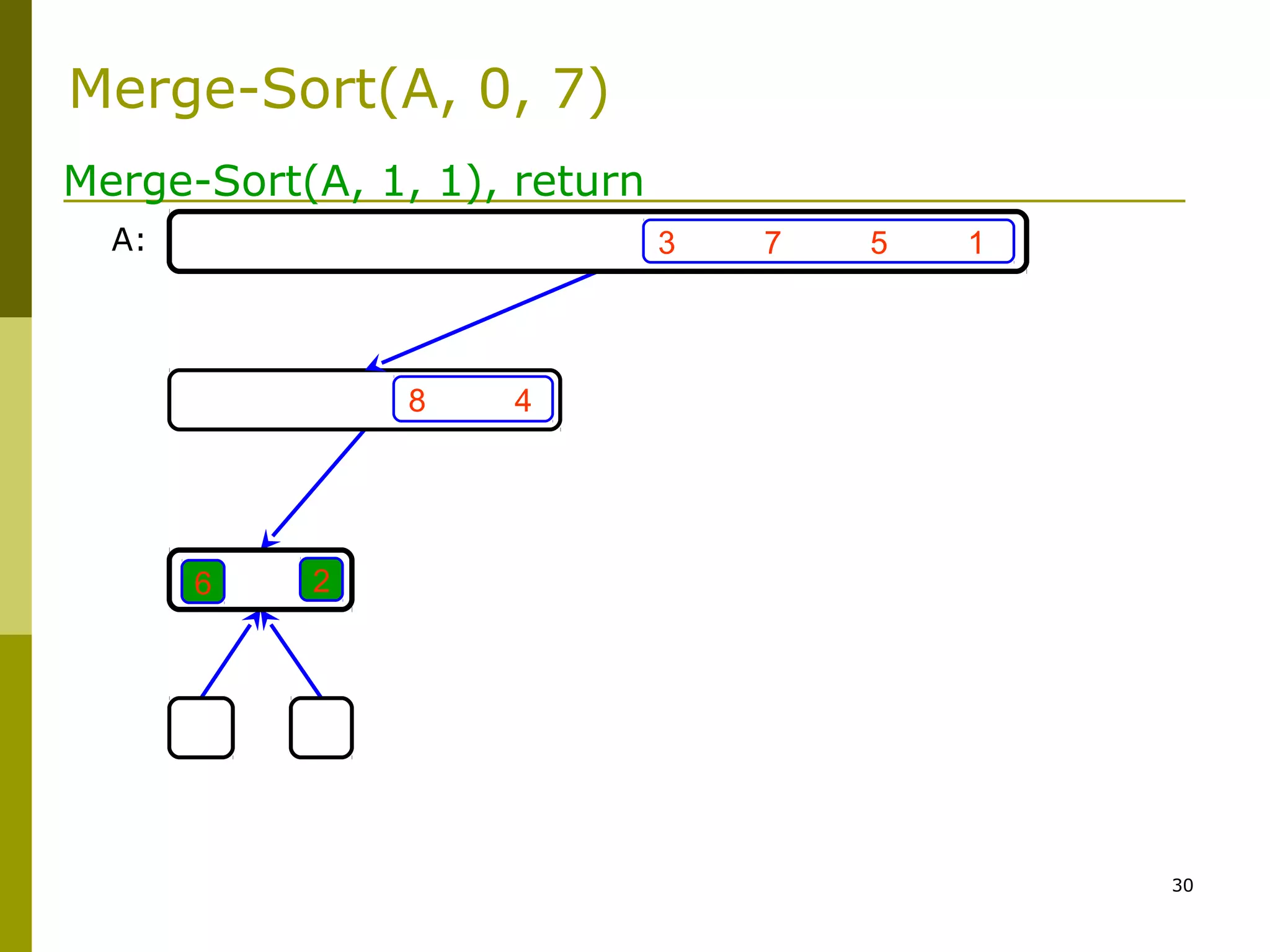
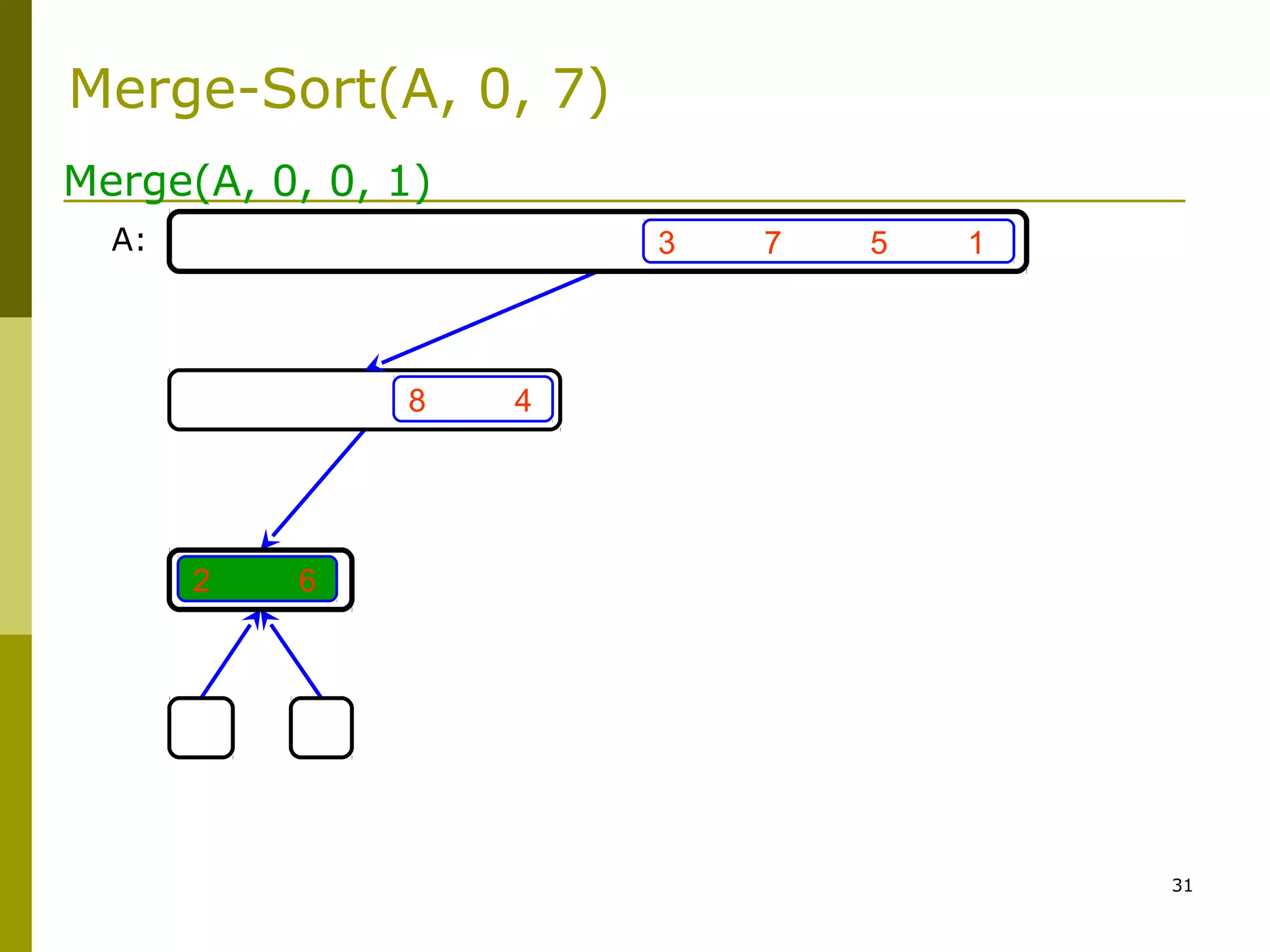
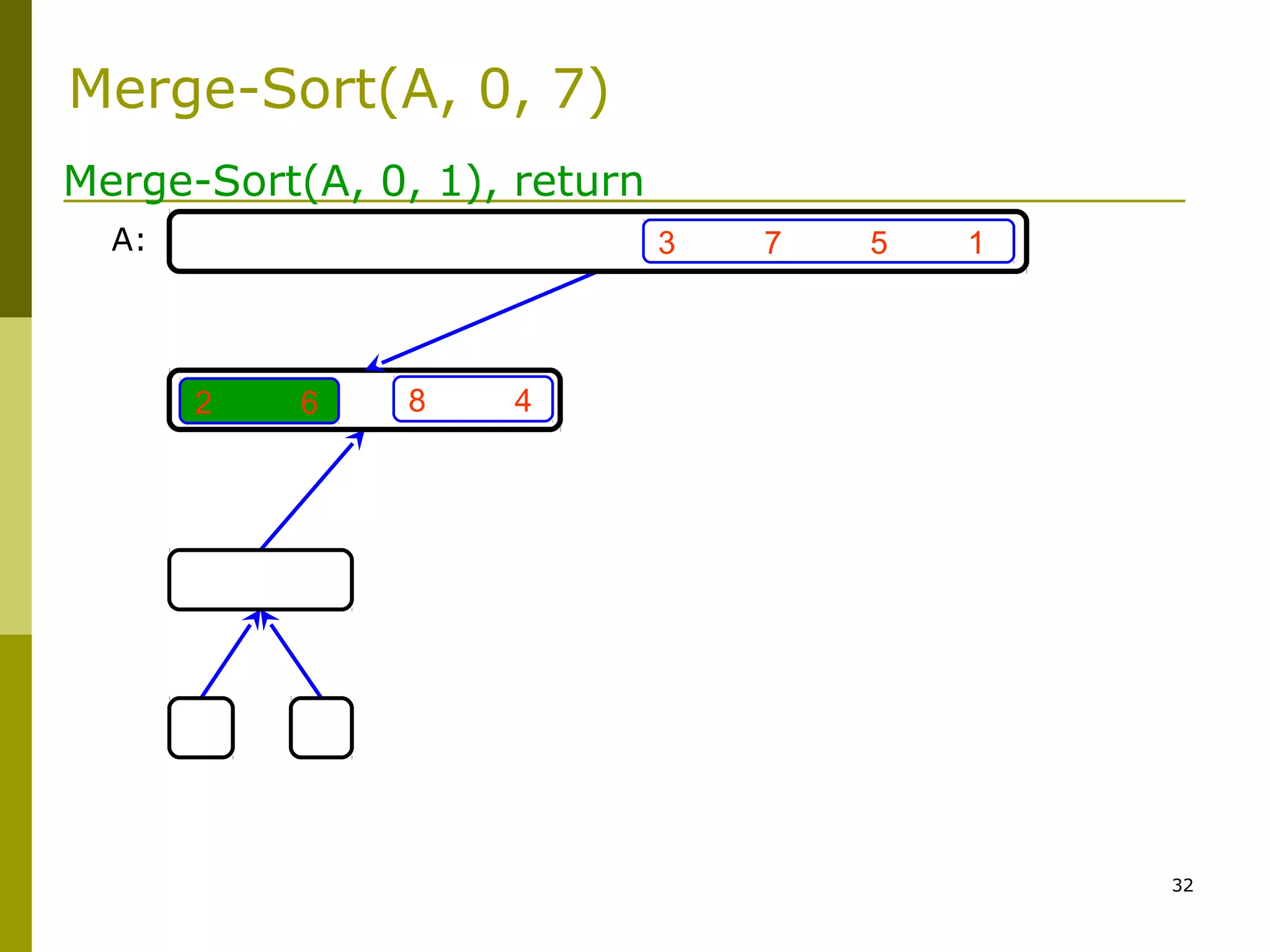
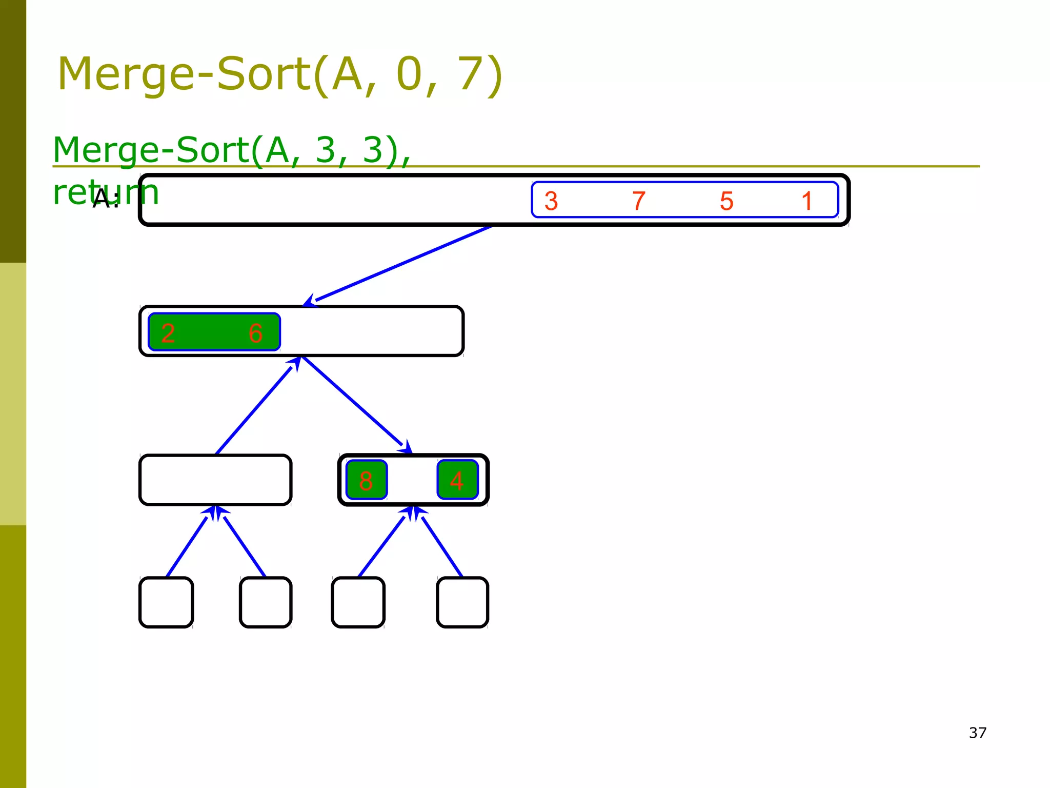
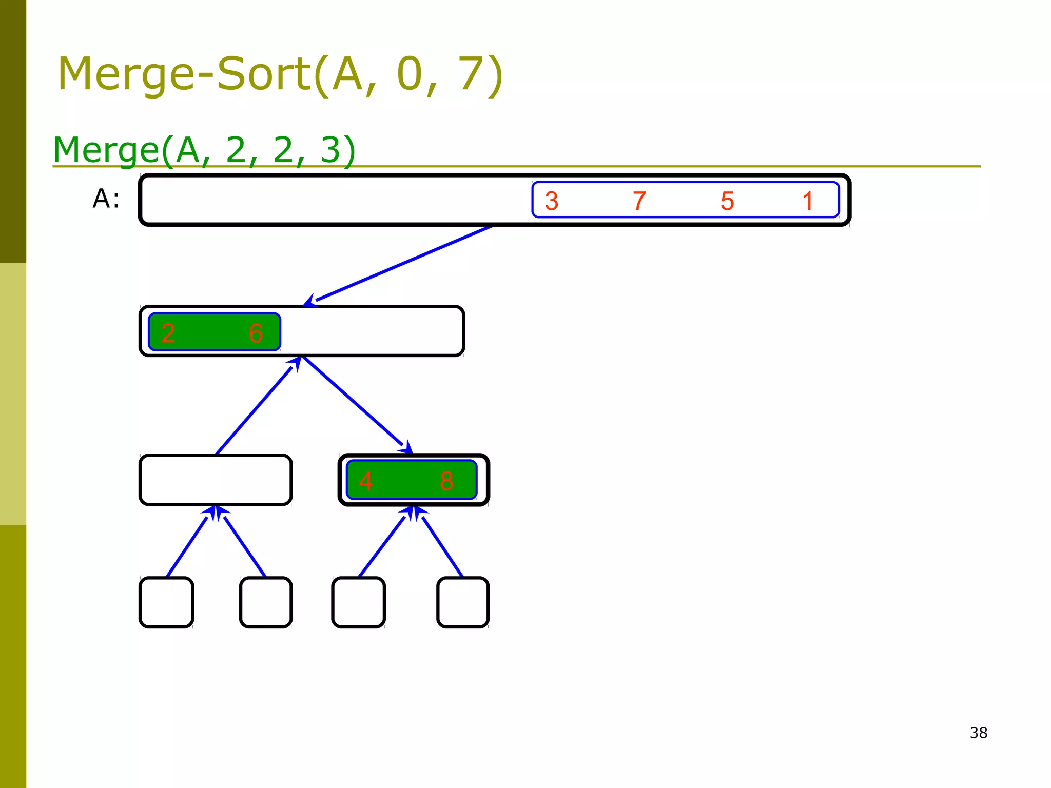
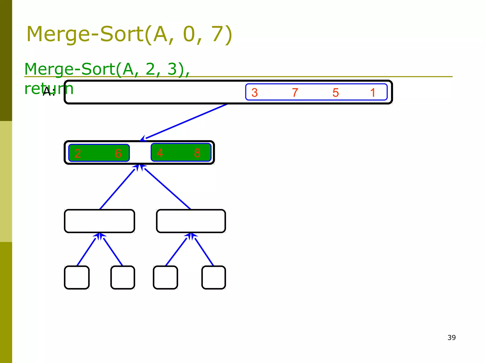
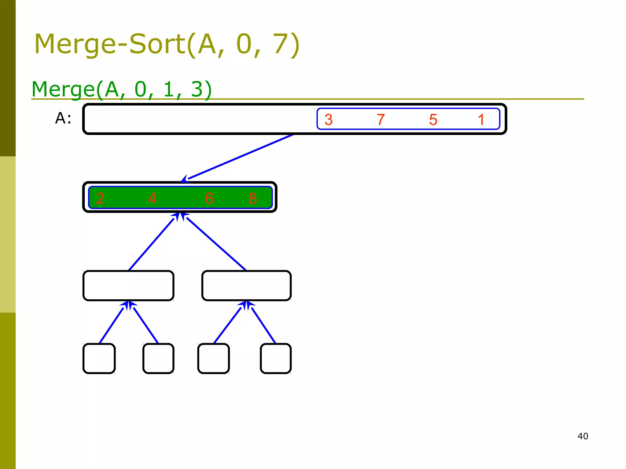
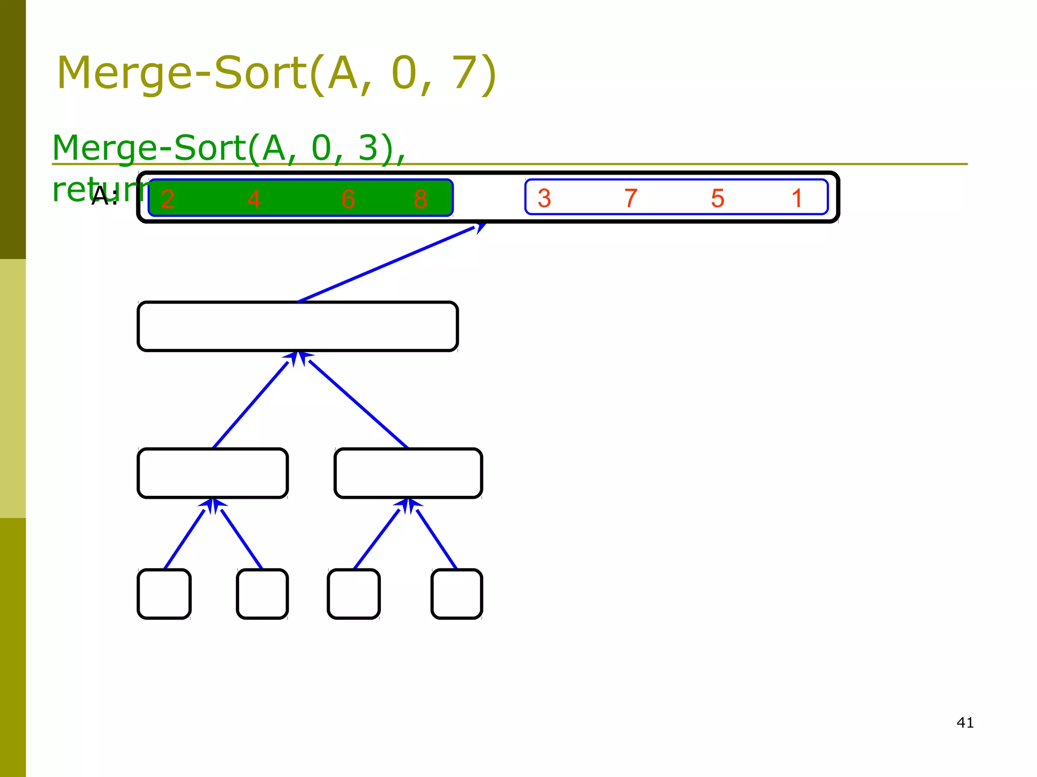
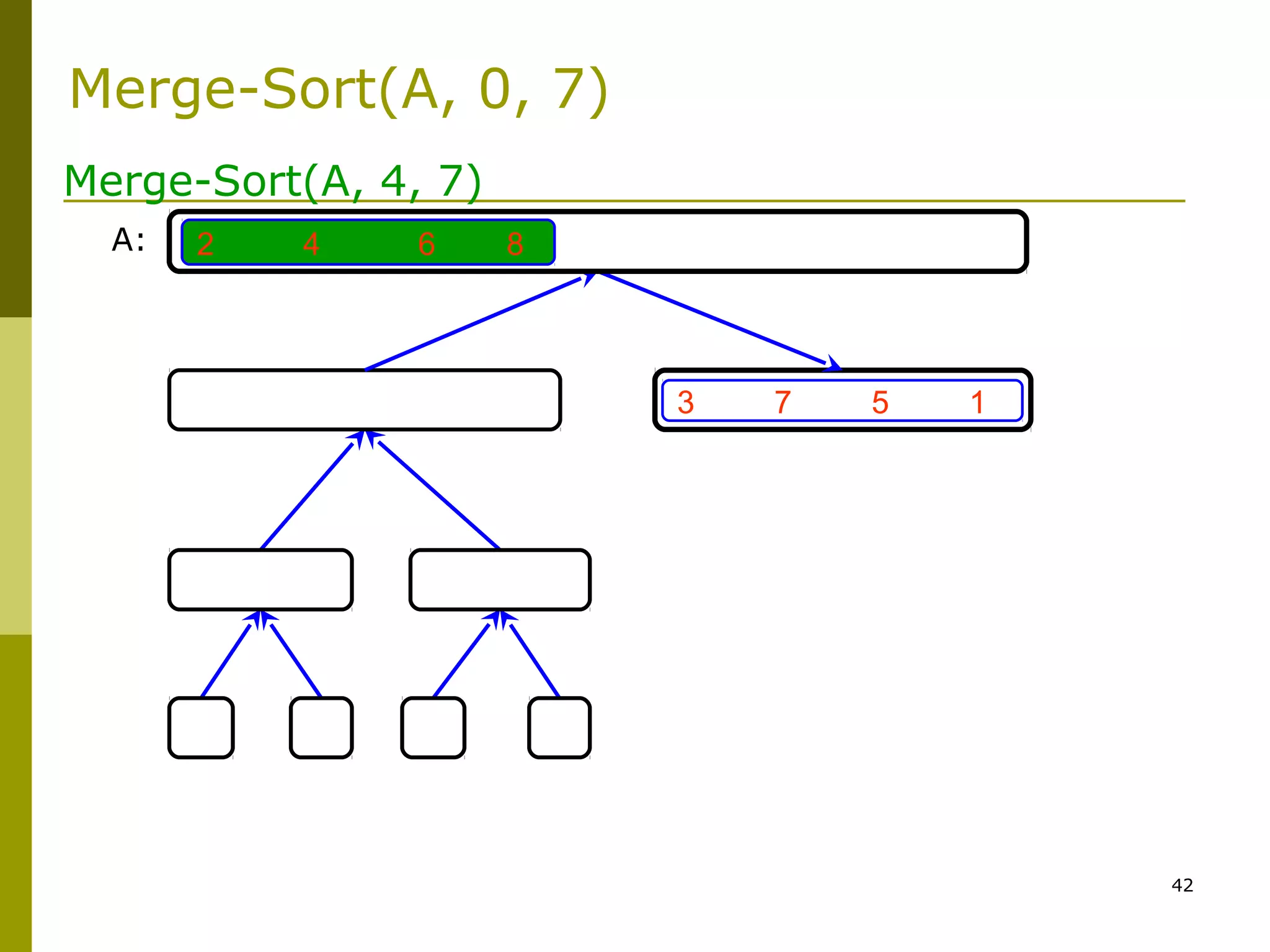
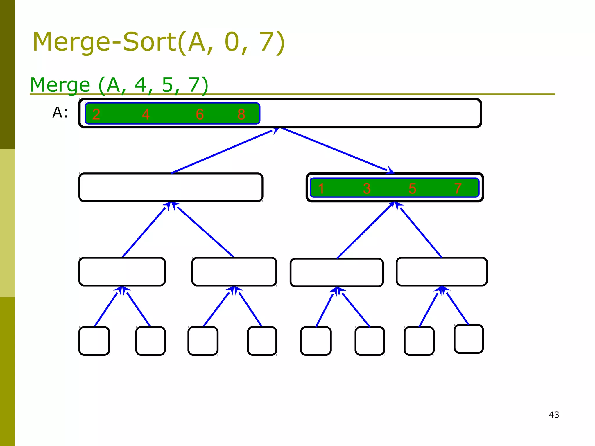
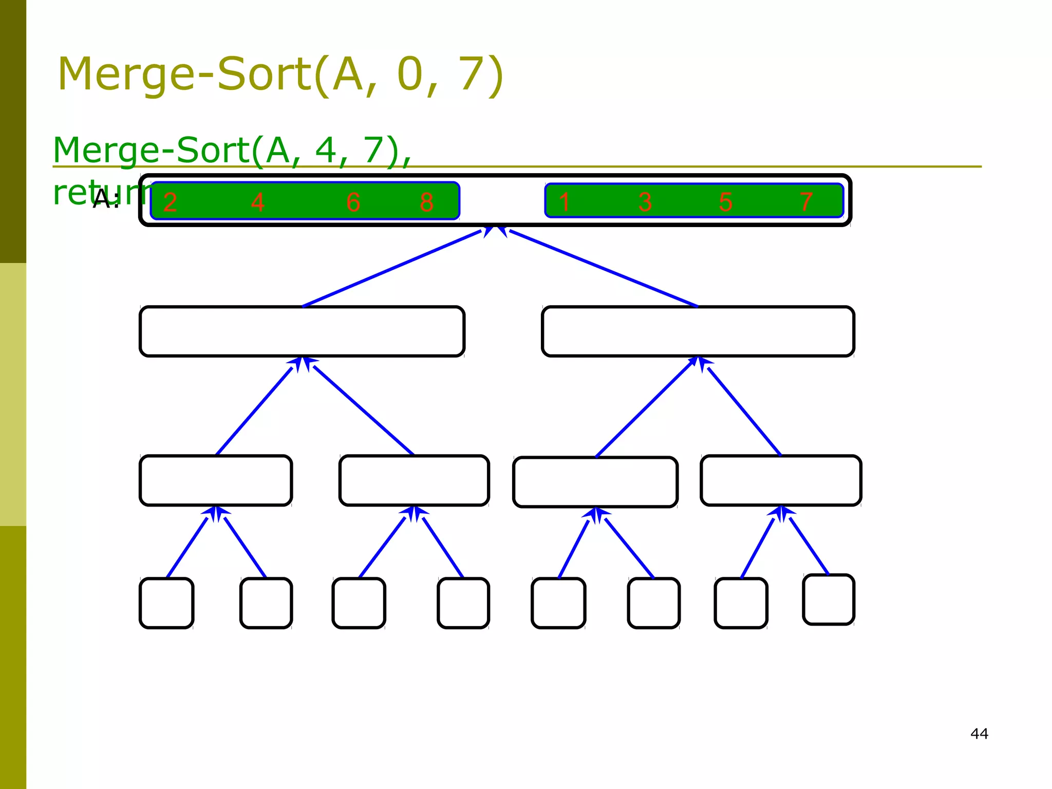
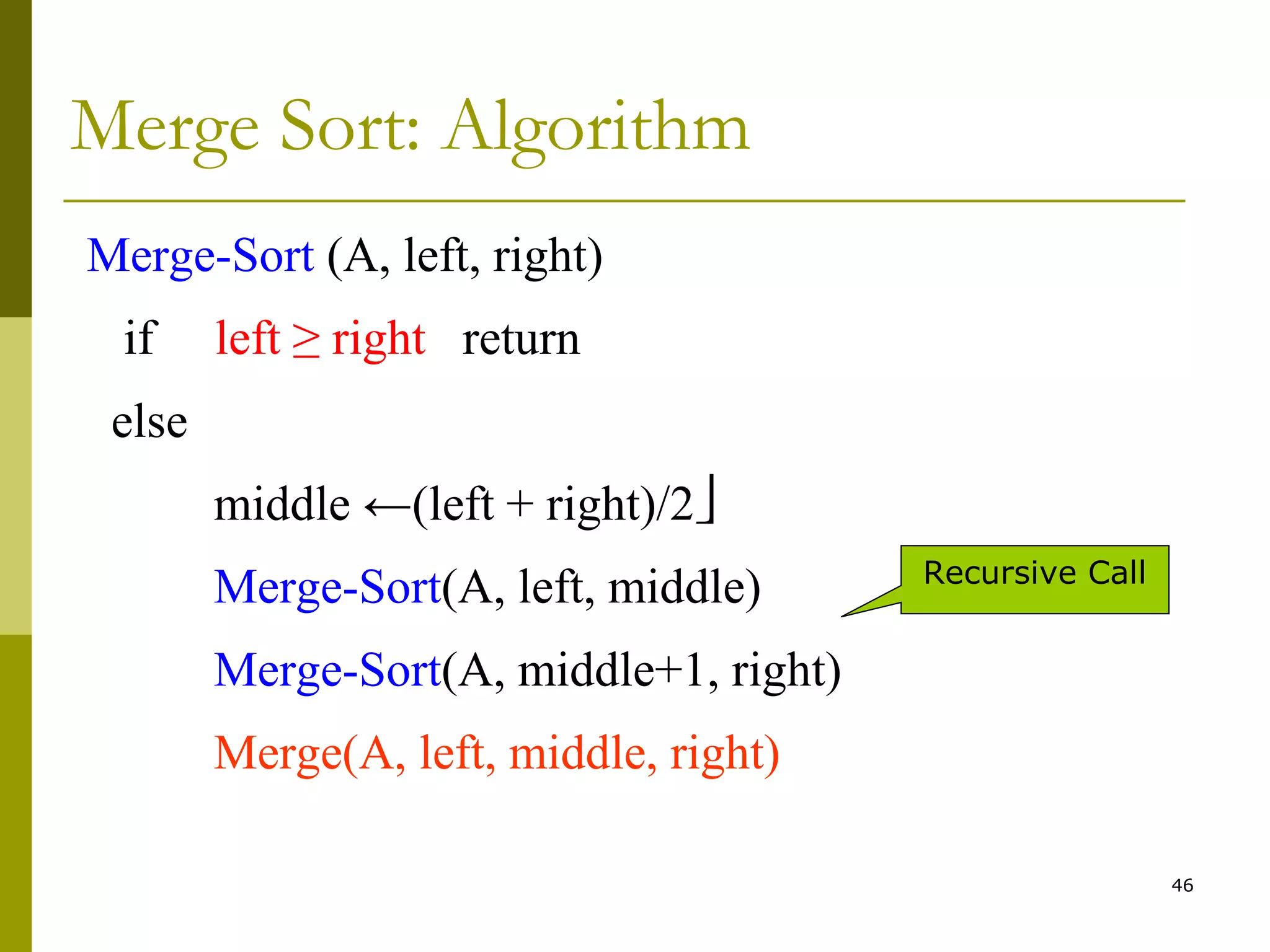
![47
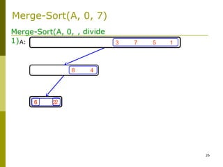
Merge(A, left, middle, right)
1. n1 ← middle – left + 1
2. n2 ← right – middle
3. create array L[n1], R[n2]
4. for i ← 0 to n1-1 do L[i] ← A[left +i]
5. for j ← 0 to n2-1 do R[j] ← A[middle+j]
6. k ← i ← j ← 0
7. while i < n1 & j < n2
8. if L[i] < R[j]
9. A[k++] ← L[i++]
10. else
11. A[k++] ← R[j++]
12. while i < n1
13. A[k++] ← L[i++]
14. while j < n2
15. A[k++] ← R[j++]
n = n1+n2
Space: n
Time : cn for some constant c](https://image.slidesharecdn.com/sorting-180808153102/85/Sorting-47-320.jpg)

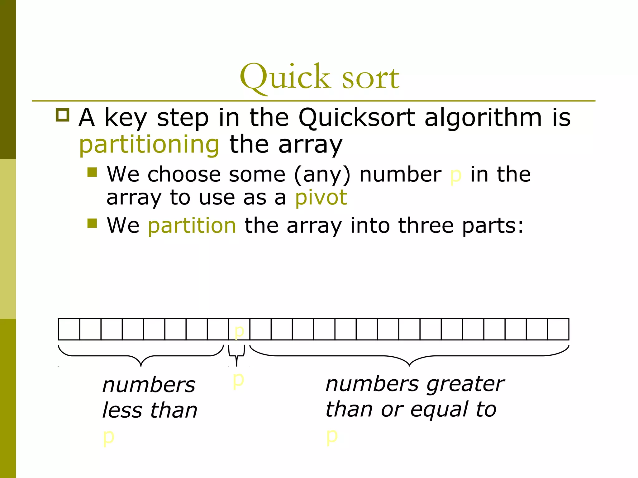
![Quick sort
To sort a[left...right]:
1. if left < right:
1.1. Partition a[left...right] such that:
all a[left...p-1] are less than a[p], and
all a[p+1...right] are >= a[p]
1.2. Quicksort a[left...p-1]
1.3. Quicksort a[p+1...right]
2. Terminate](https://image.slidesharecdn.com/sorting-180808153102/75/Sorting-9-2048.jpg)
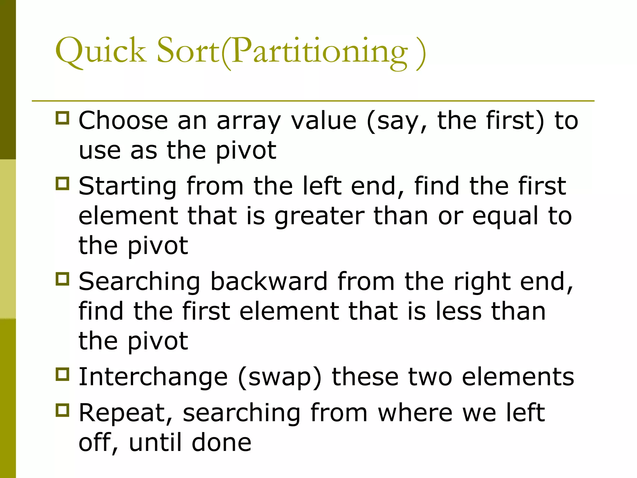
![Partitioning
To partition a[left...right]:
1. Set p = a[left], l = left + 1, r = right;
2. while l < r, do
2.1. while l < right && a[l] < p { l = l + 1 }
2.2. while r > left && a[r] >= p { r = r – 1}
2.3. if l < r { swap a[l] and a[r] }
3. a[left] = a[r]; a[r] = p;
4. Terminate](https://image.slidesharecdn.com/sorting-180808153102/75/Sorting-10-2048.jpg)

![13
A[middle]A[middle]A[left]A[left]
SortedSorted
FirstPartFirstPart
SortedSorted
SecondPartSecondPart
Merge-Sort: Merge
A[right]A[right]
mergemerge
A:A:
A:A:
SortedSorted](https://image.slidesharecdn.com/sorting-180808153102/75/Sorting-13-2048.jpg)

![47
Merge(A, left, middle, right)
1. n1 ← middle – left + 1
2. n2 ← right – middle
3. create array L[n1], R[n2]
4. for i ← 0 to n1-1 do L[i] ← A[left +i]
5. for j ← 0 to n2-1 do R[j] ← A[middle+j]
6. k ← i ← j ← 0
7. while i < n1 & j < n2
8. if L[i] < R[j]
9. A[k++] ← L[i++]
10. else
11. A[k++] ← R[j++]
12. while i < n1
13. A[k++] ← L[i++]
14. while j < n2
15. A[k++] ← R[j++]
n = n1+n2
Space: n
Time : cn for some constant c](https://image.slidesharecdn.com/sorting-180808153102/75/Sorting-47-2048.jpg)

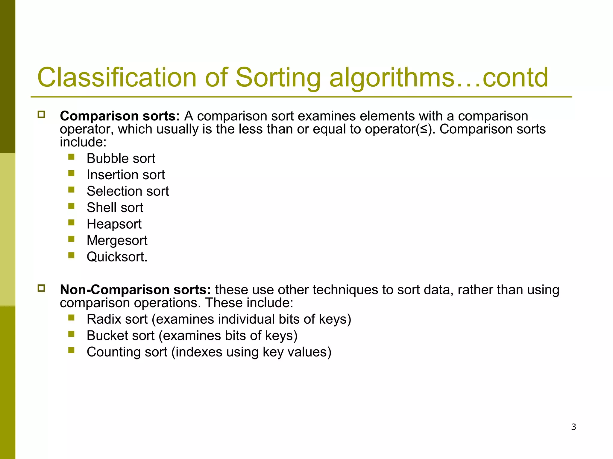
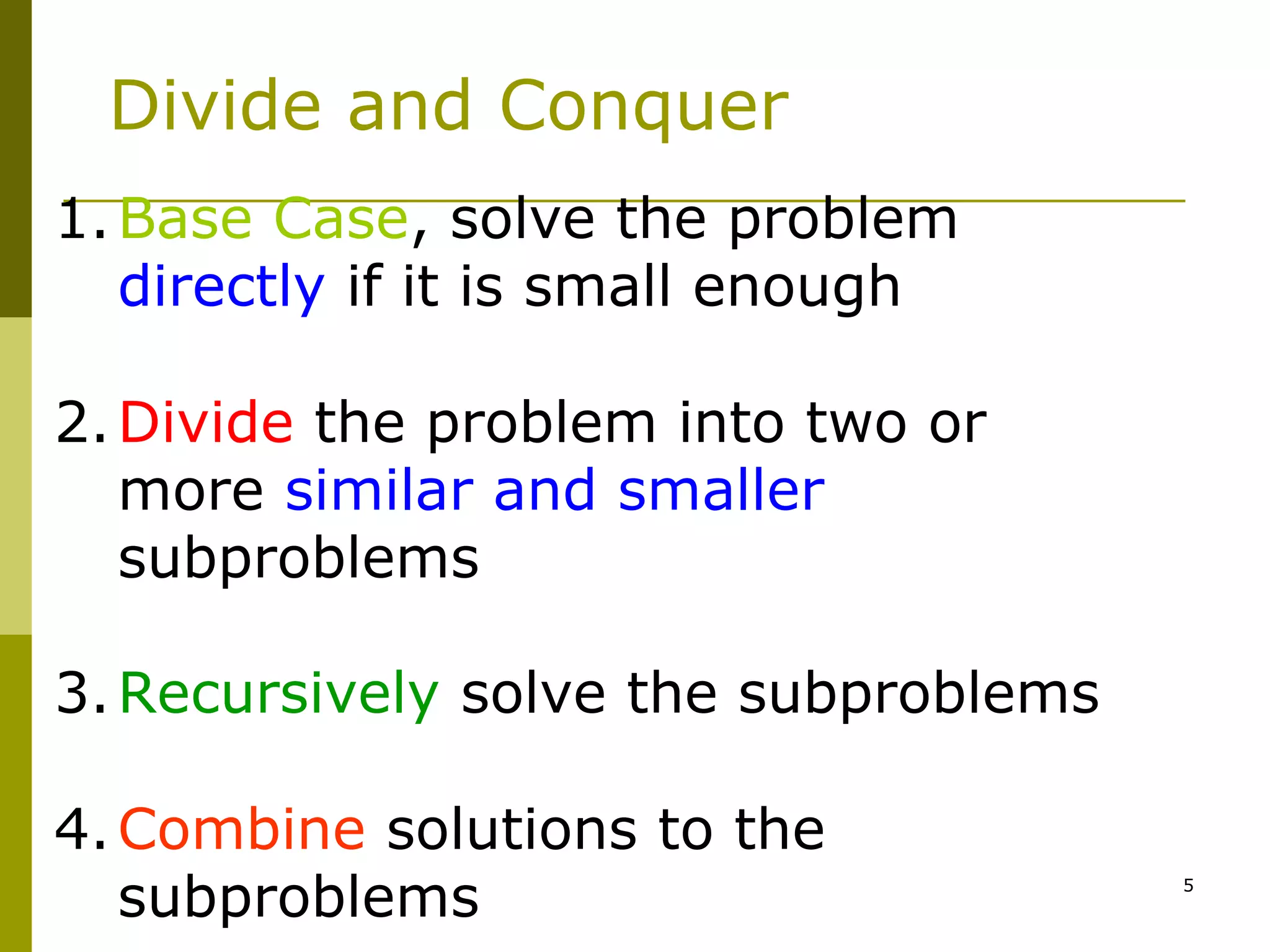
The document provides an overview of sorting algorithms, emphasizing their classification based on criteria such as computational complexity, memory usage, and internal methods. It further details specific algorithms like quicksort and mergesort, explaining their mechanisms and processes. Efficient sorting is highlighted as a crucial step to optimize other algorithms and solve various problems.


![UNIT V Searching Sorting Hashing Techniques [Autosaved].pptx](https://cdn.slidesharecdn.com/ss_thumbnails/unitvsearchingsortinghashingtechniquesautosaved-241126054304-95a69c51-thumbnail.jpg?width=600ounds&width=560&fit=bounds)

![UNIT V Searching Sorting Hashing Techniques [Autosaved].pptx](https://cdn.slidesharecdn.com/ss_thumbnails/unitvsearchingsortinghashingtechniquesautosaved-241014040608-74caa0f6-thumbnail.jpg?width=600ounds&width=560&fit=bounds)


