The document discusses several optimization searching strategies:
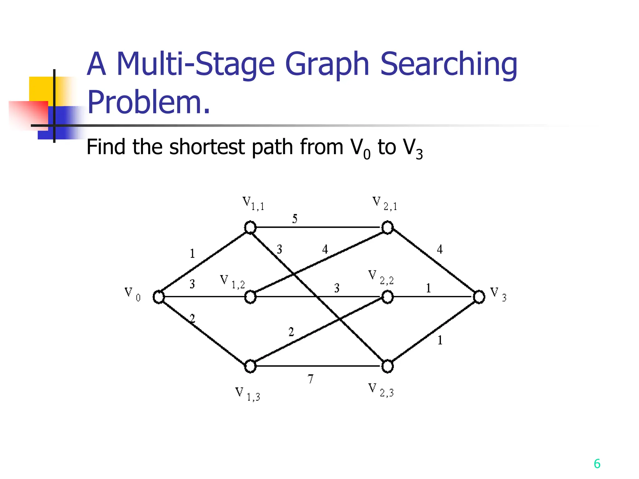
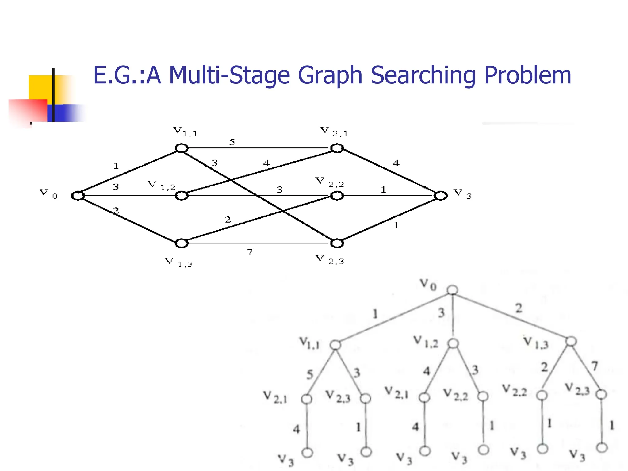
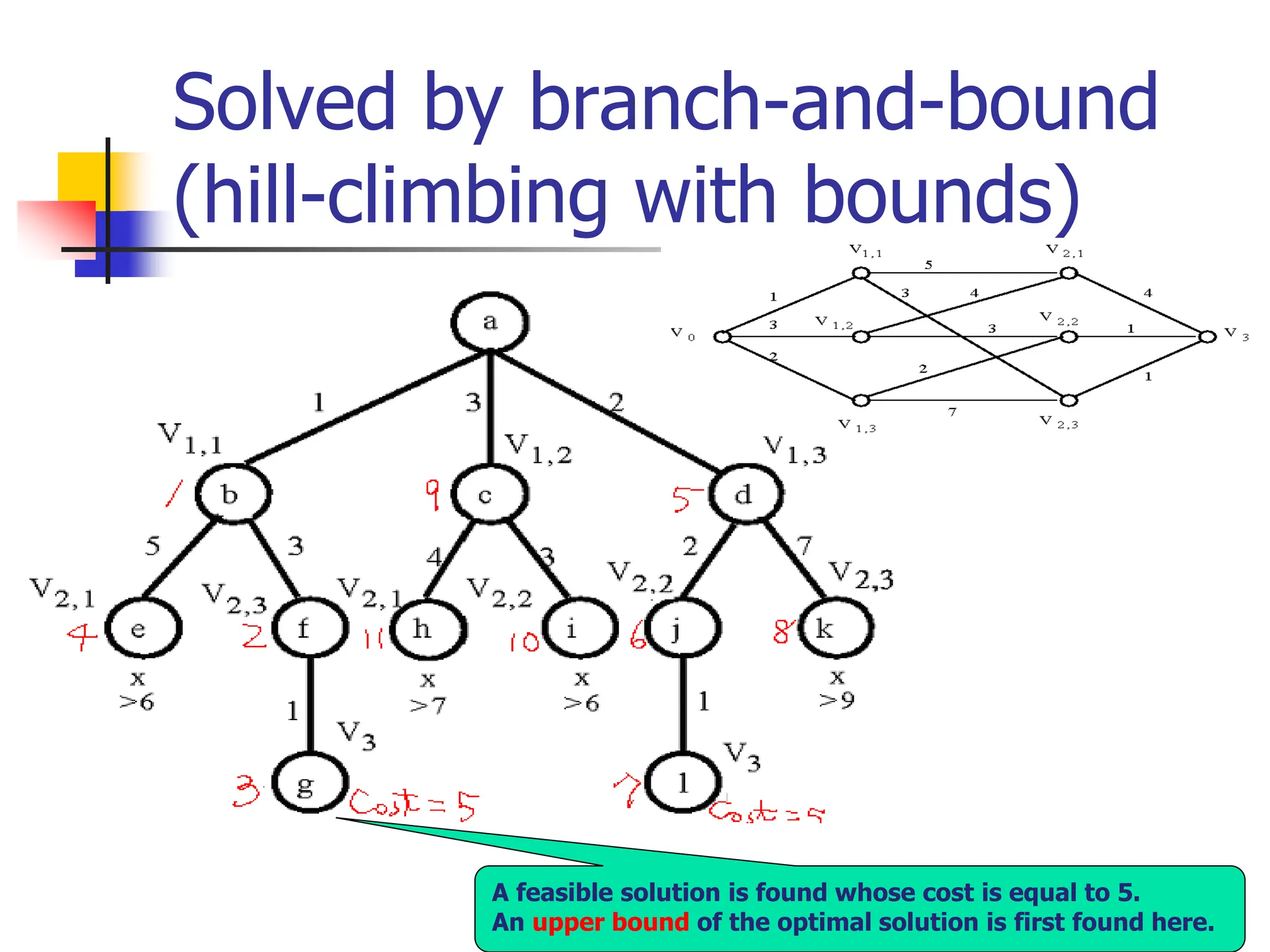
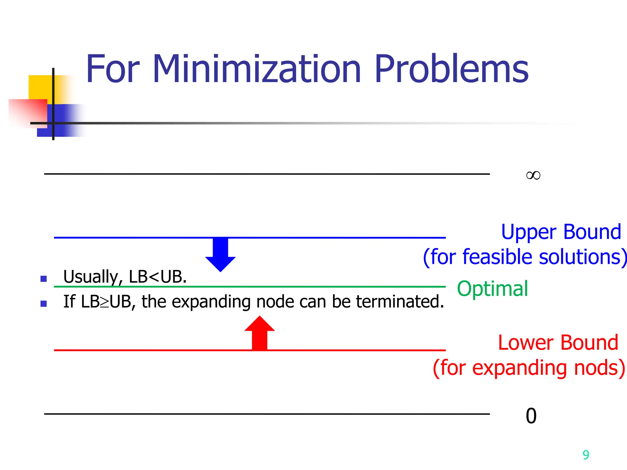
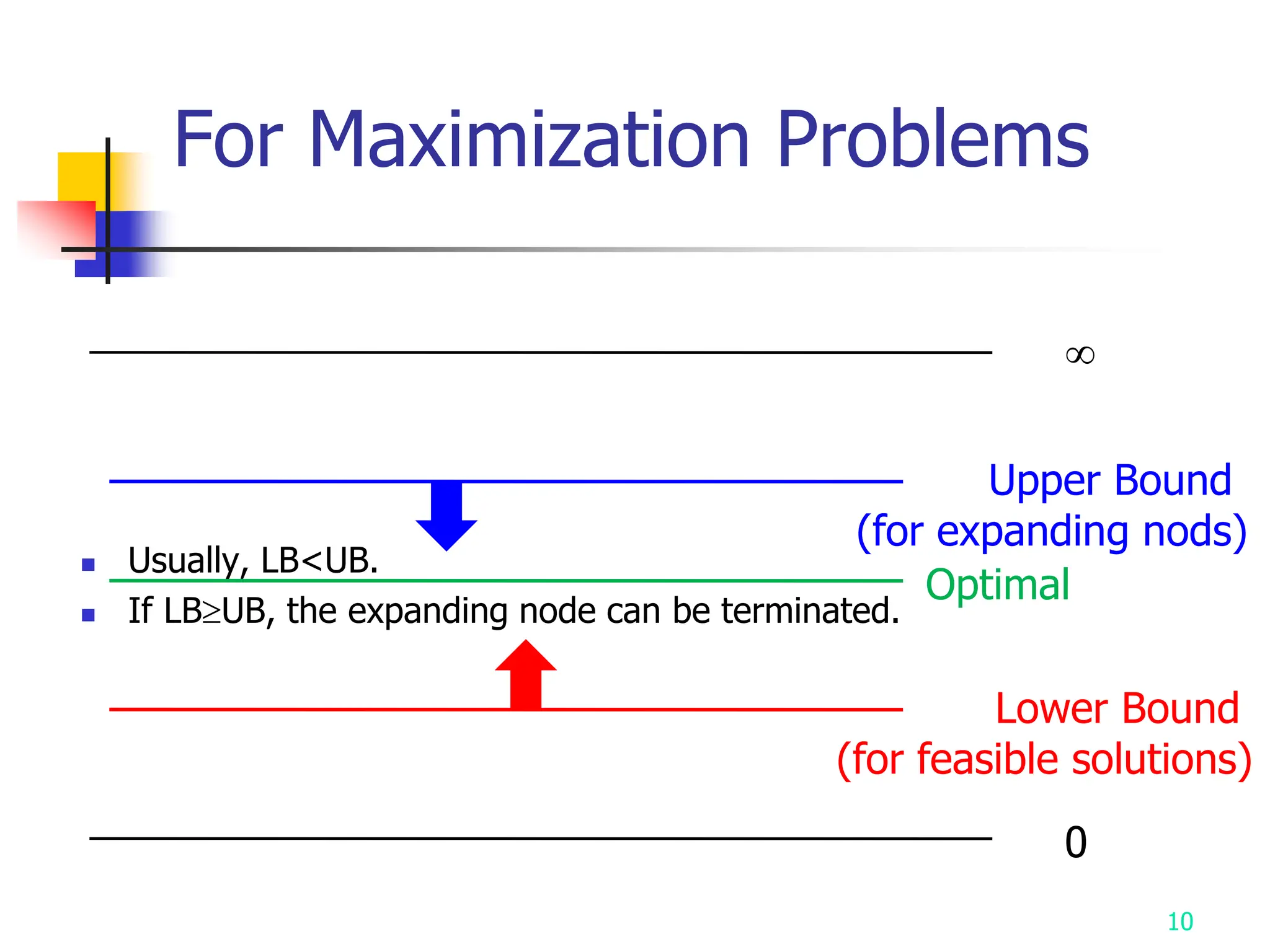
1) Branch and bound strategy uses two mechanisms - branching to generate solution space and bounding to prune branches where lower bound exceeds upper bound. It is efficient on average but worst case is exponential.
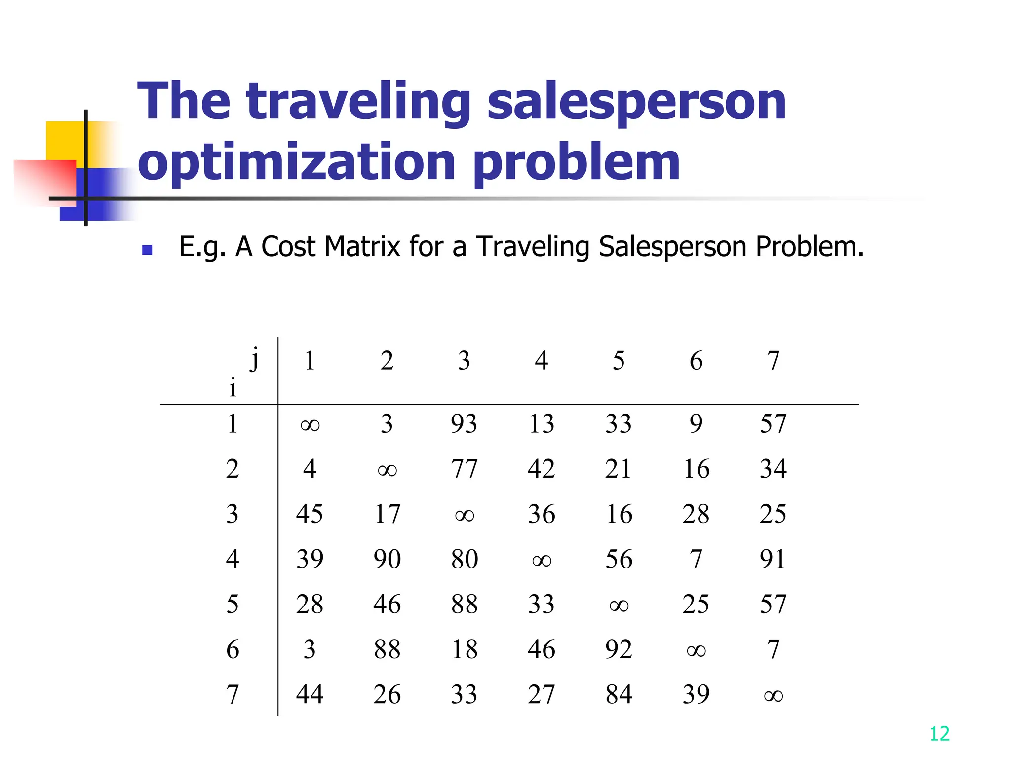
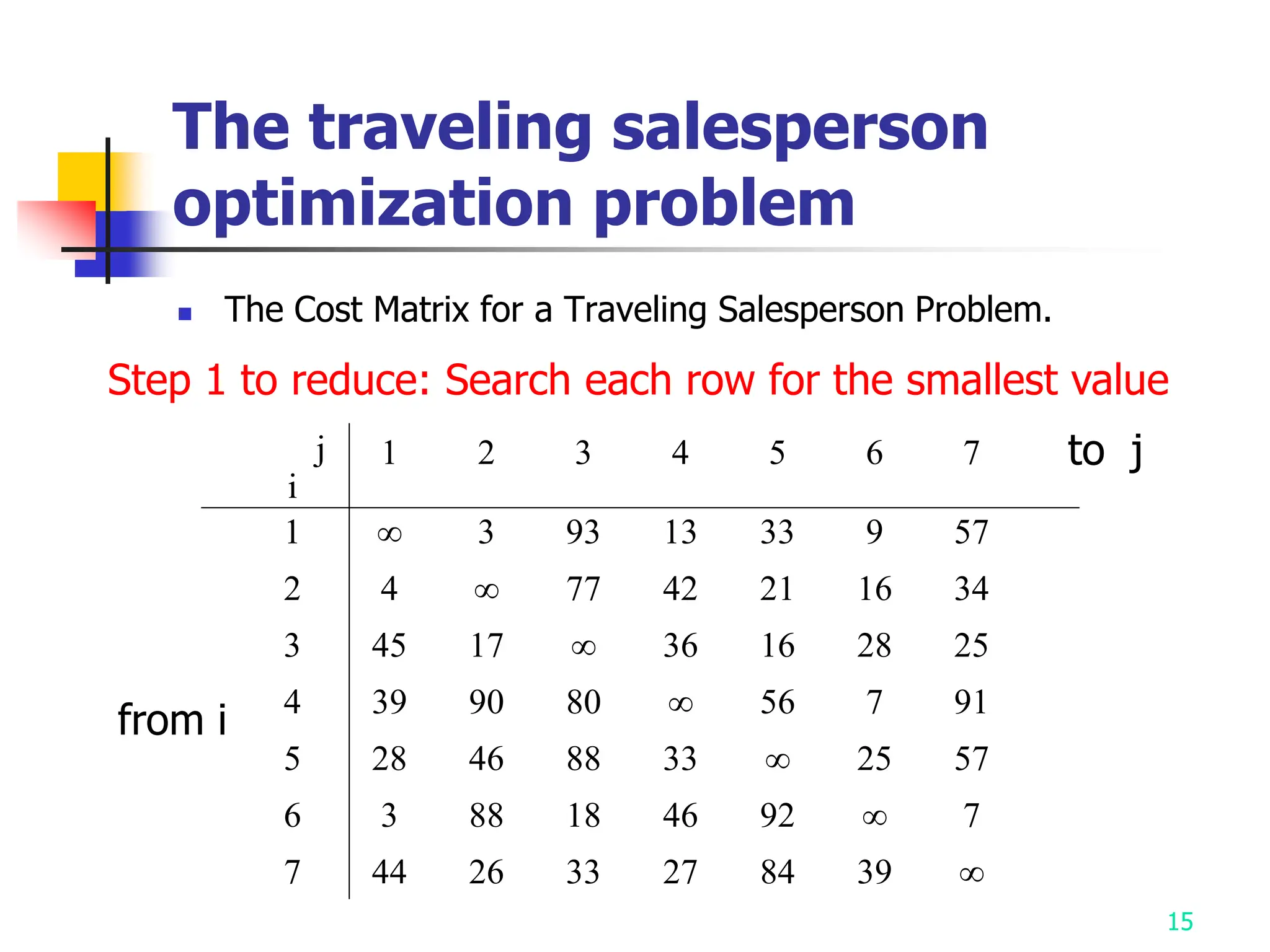
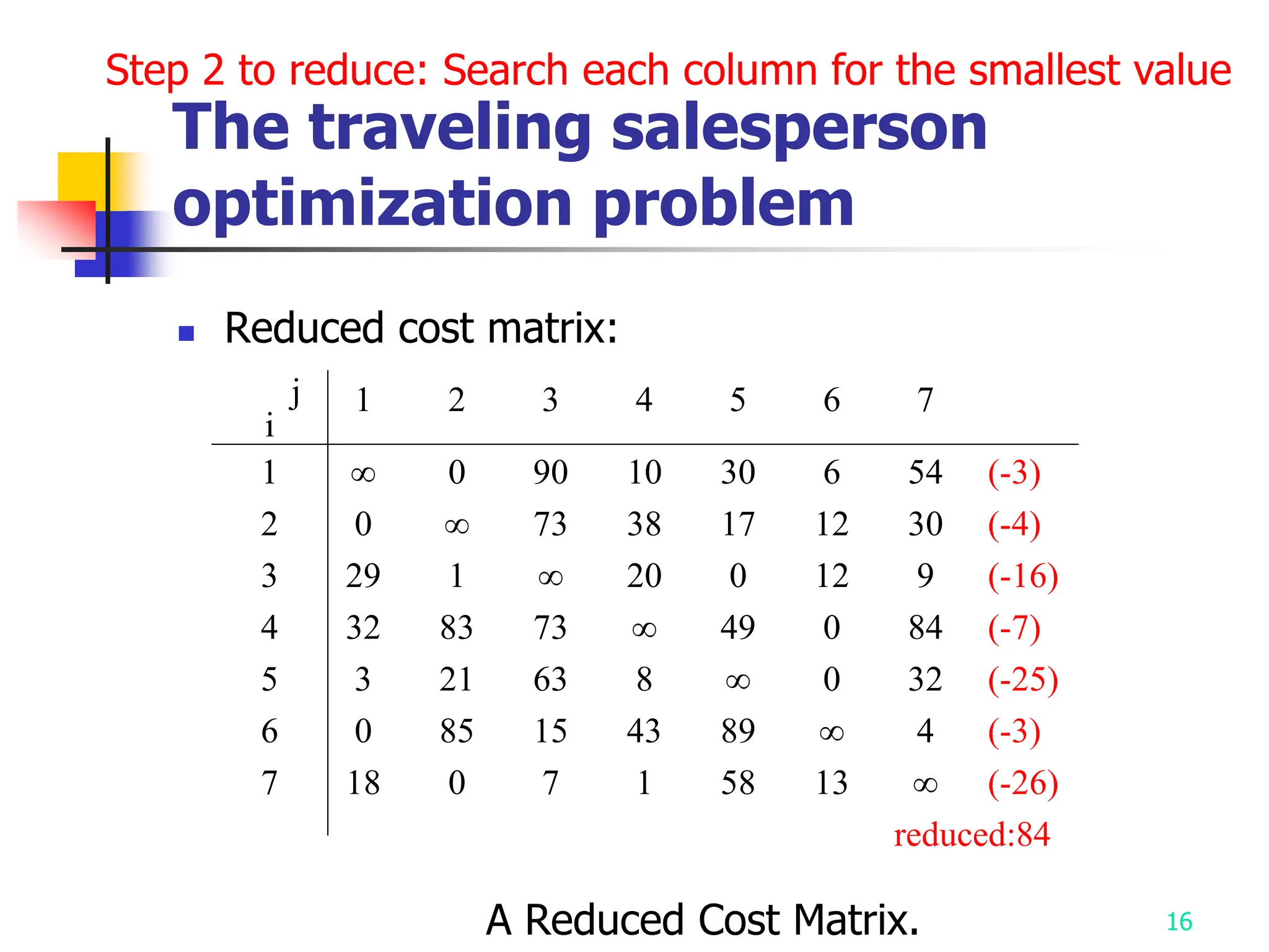
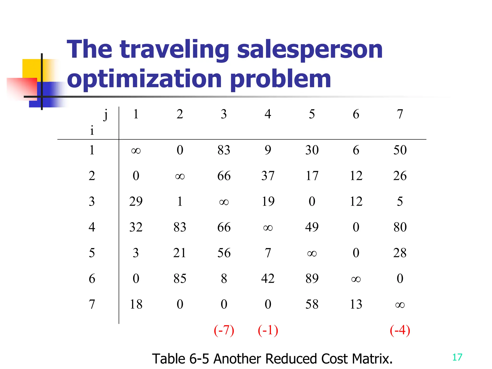
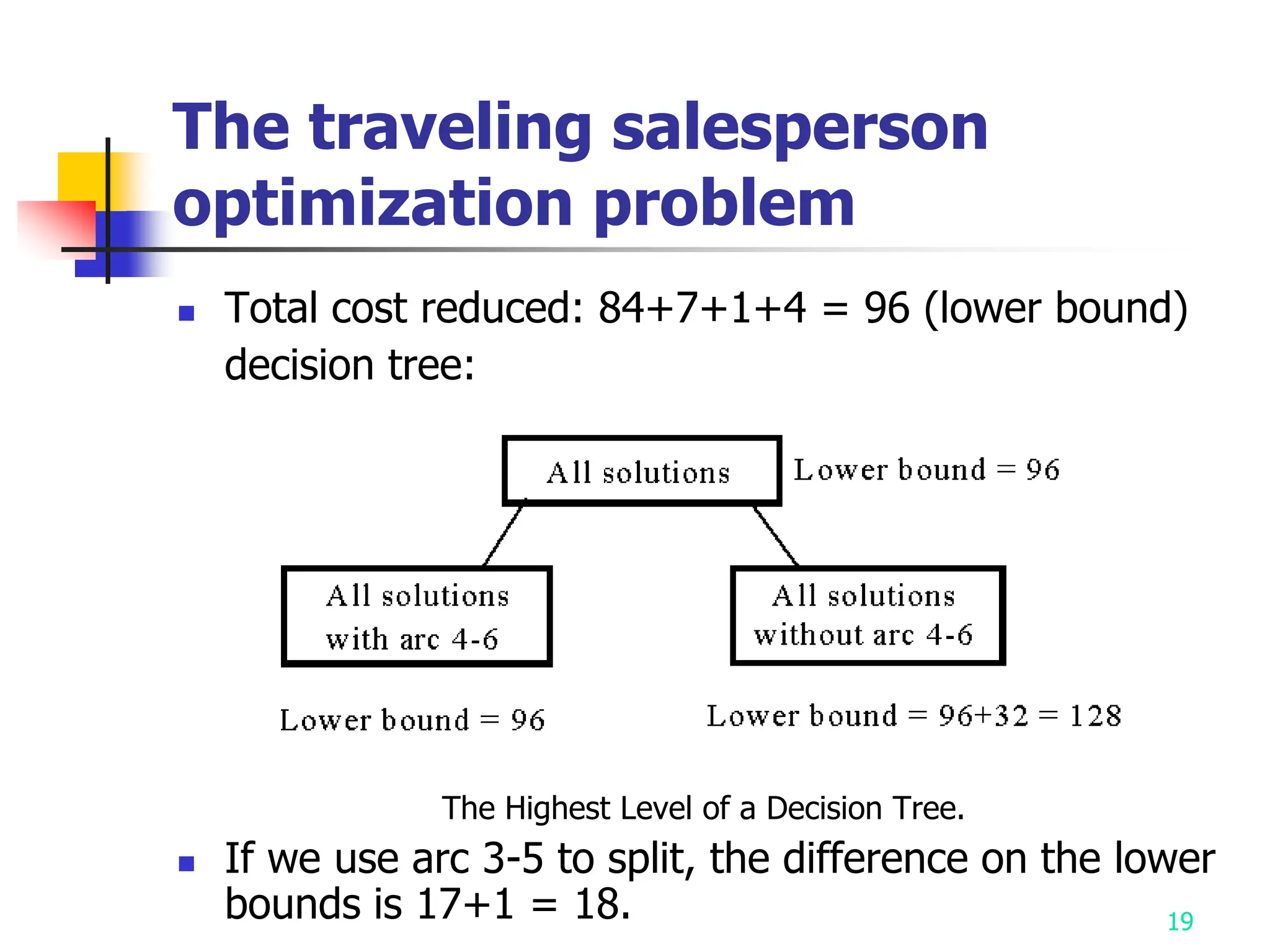
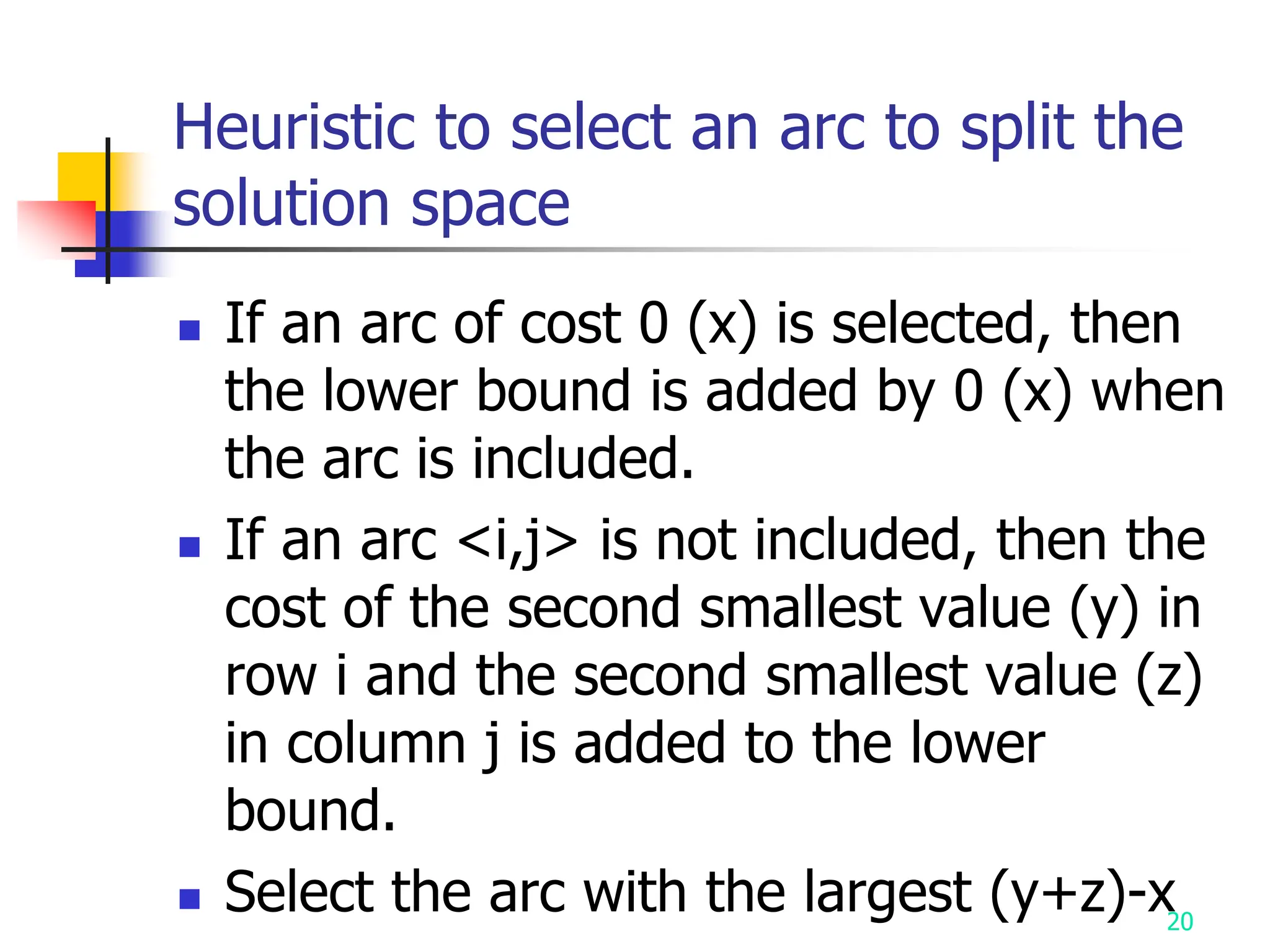
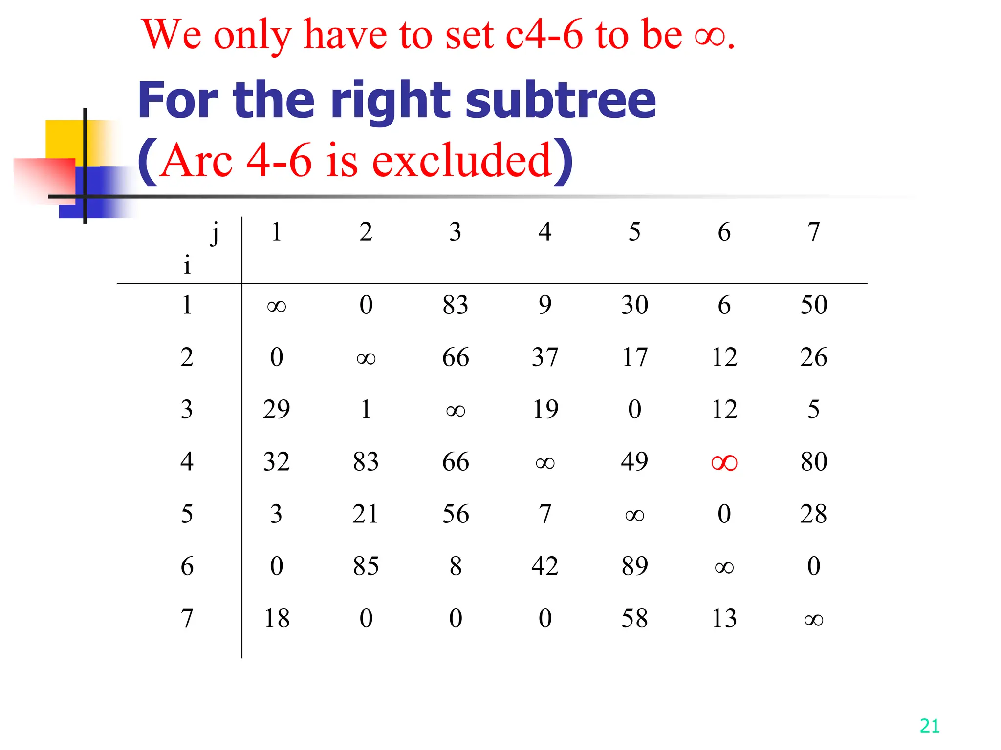
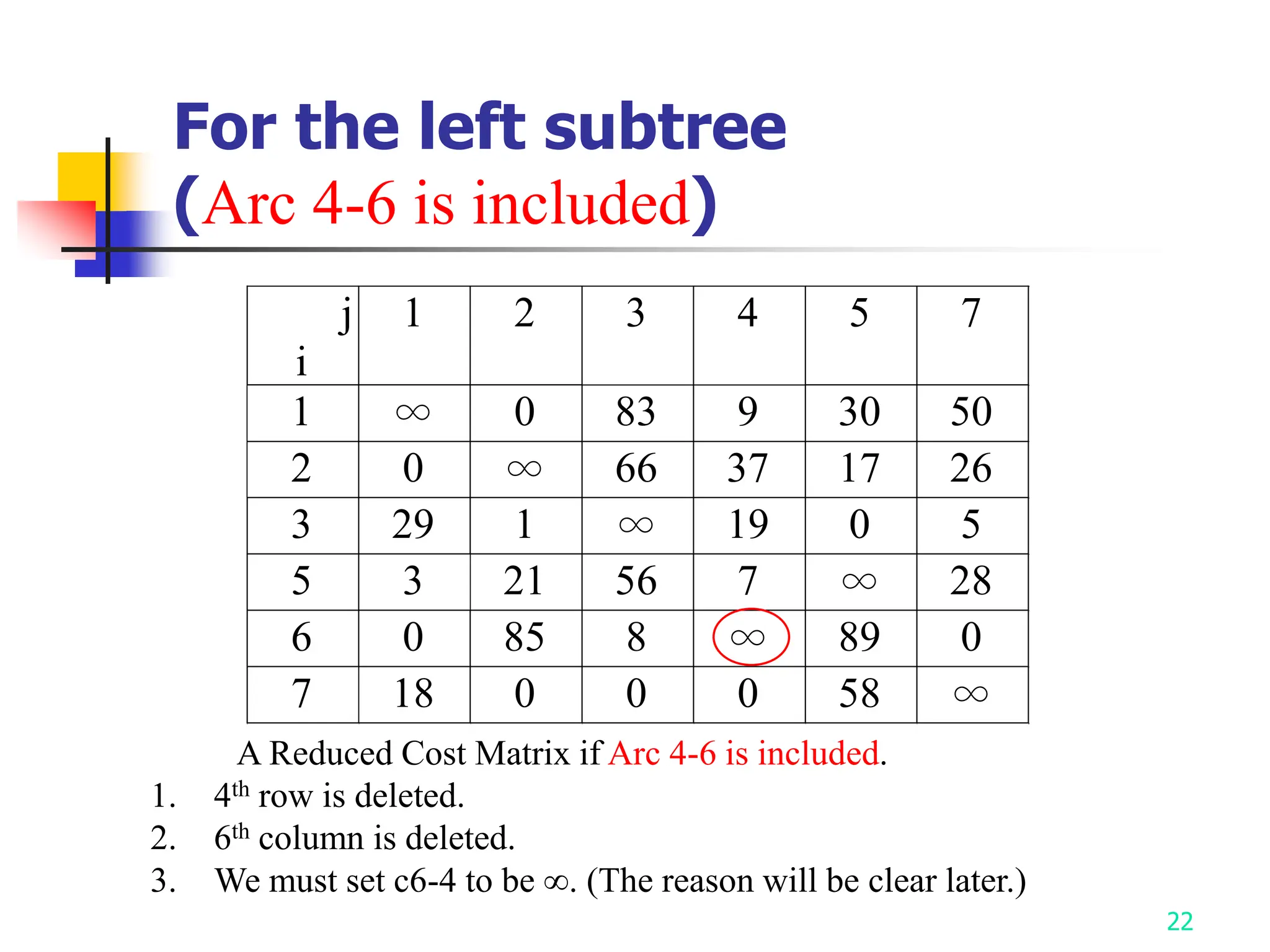
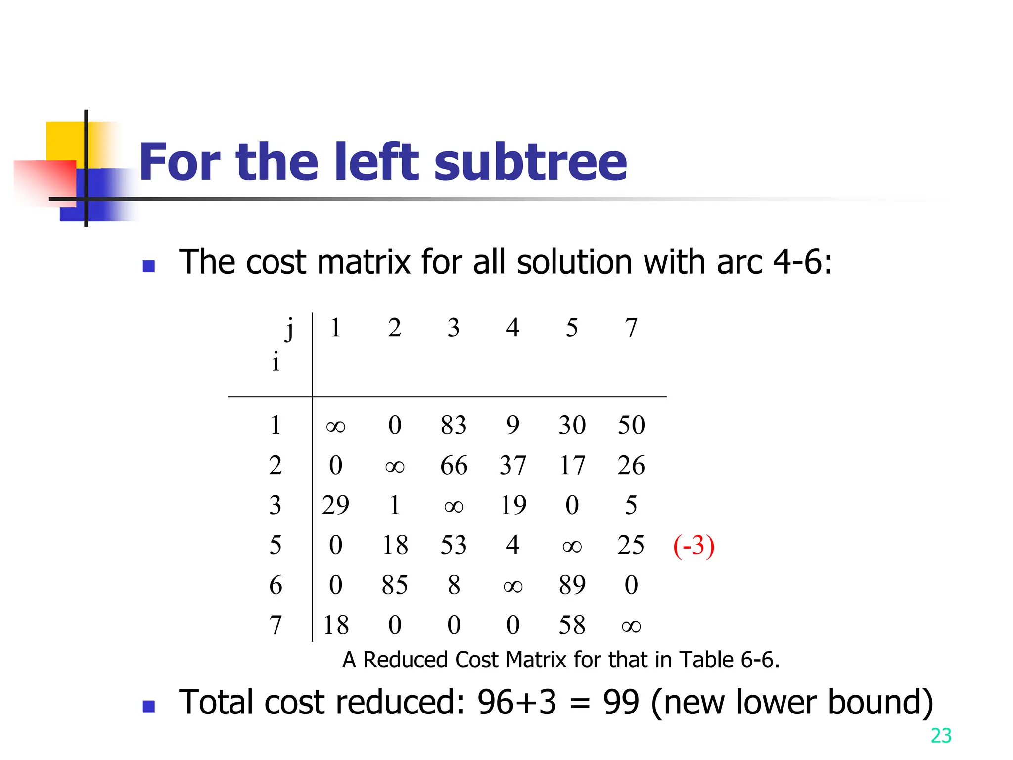
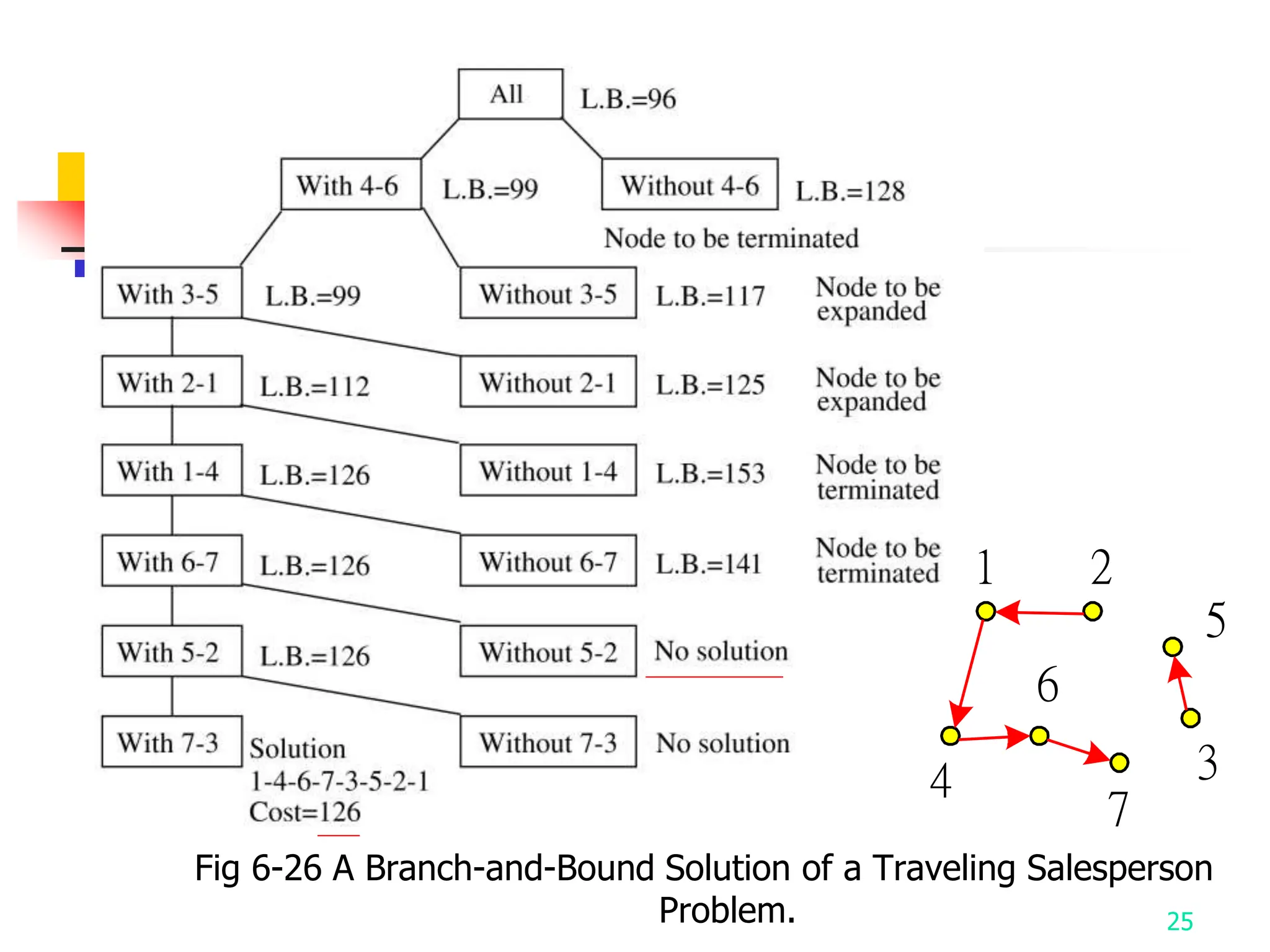
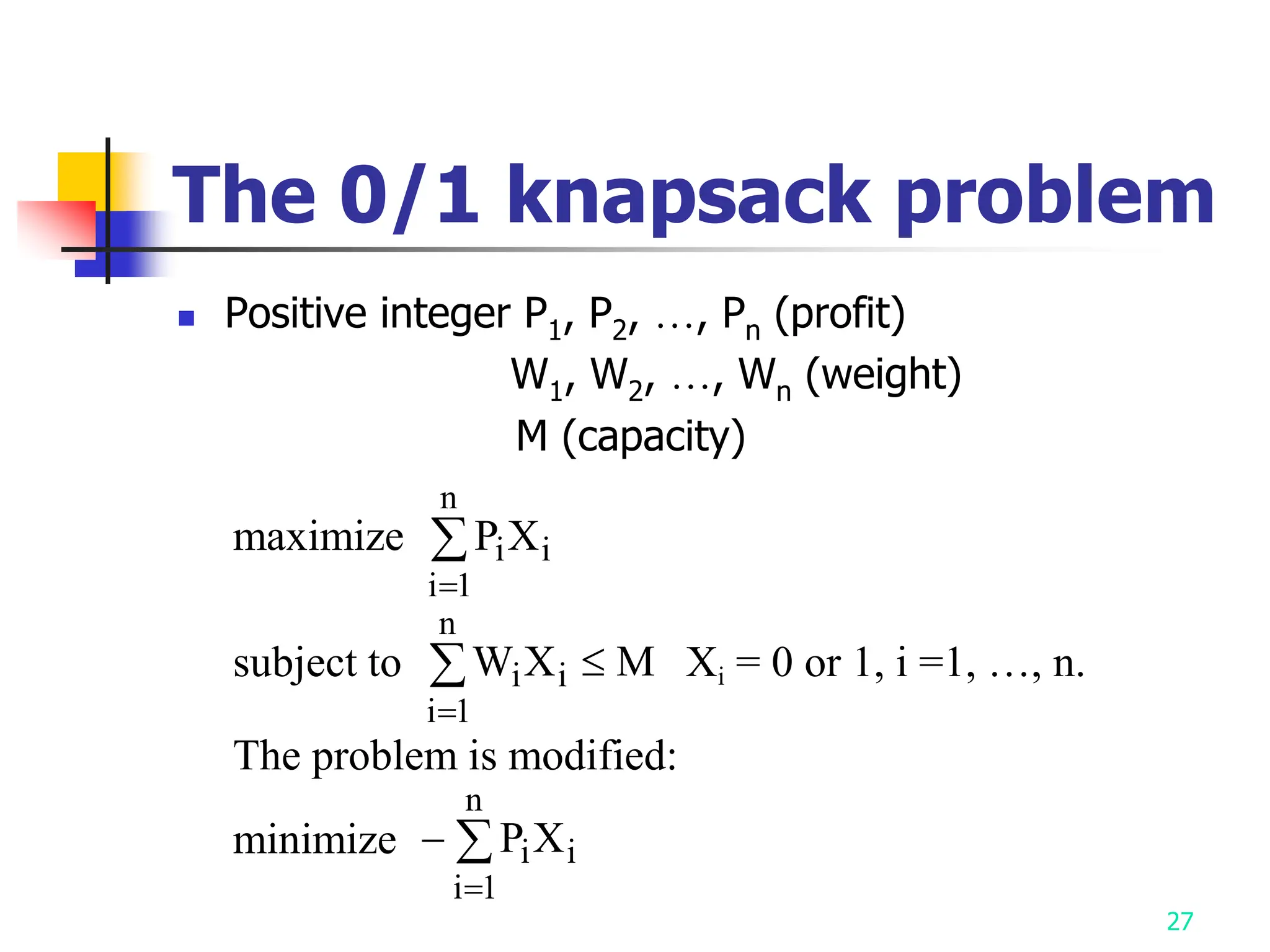
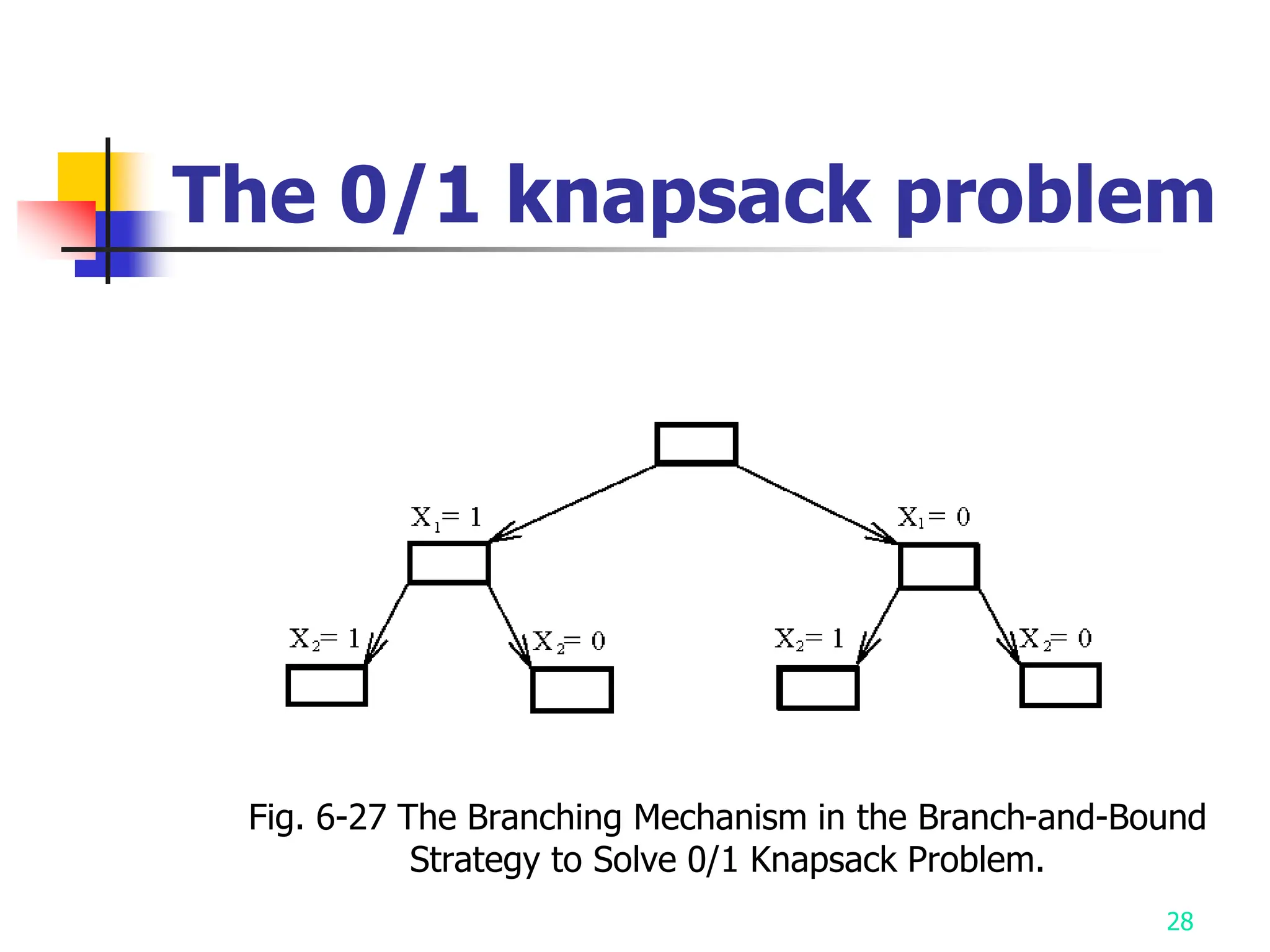
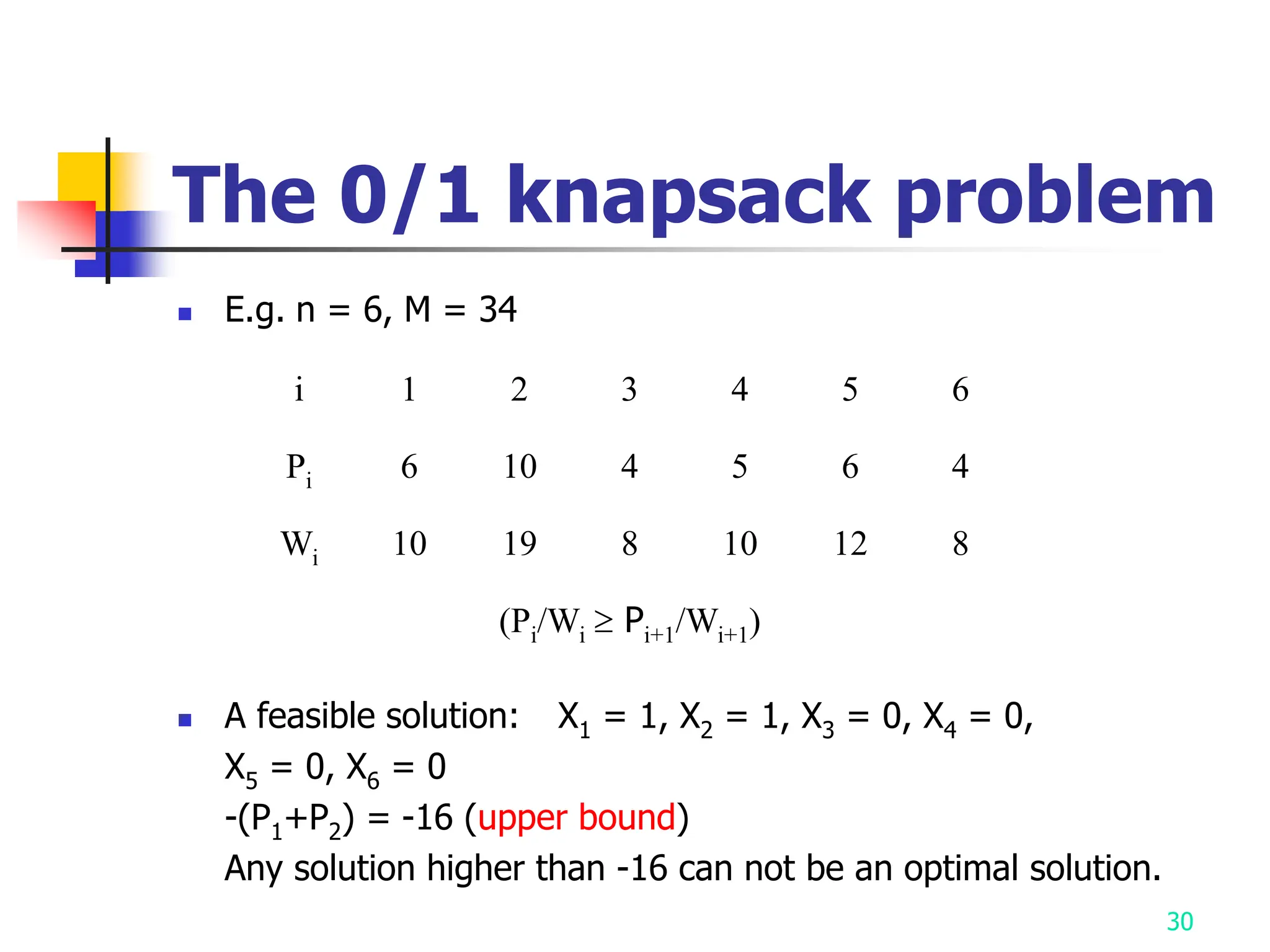
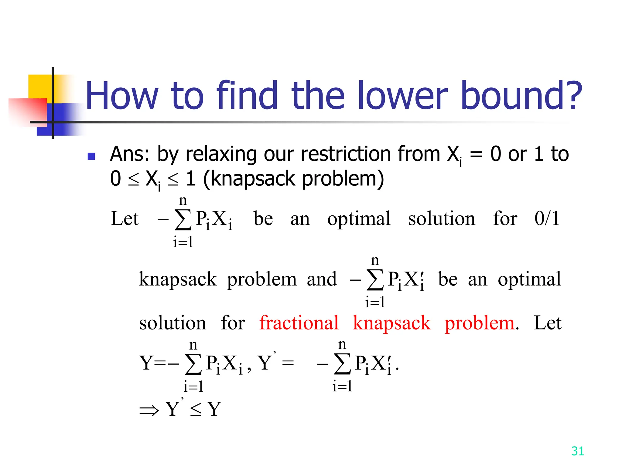
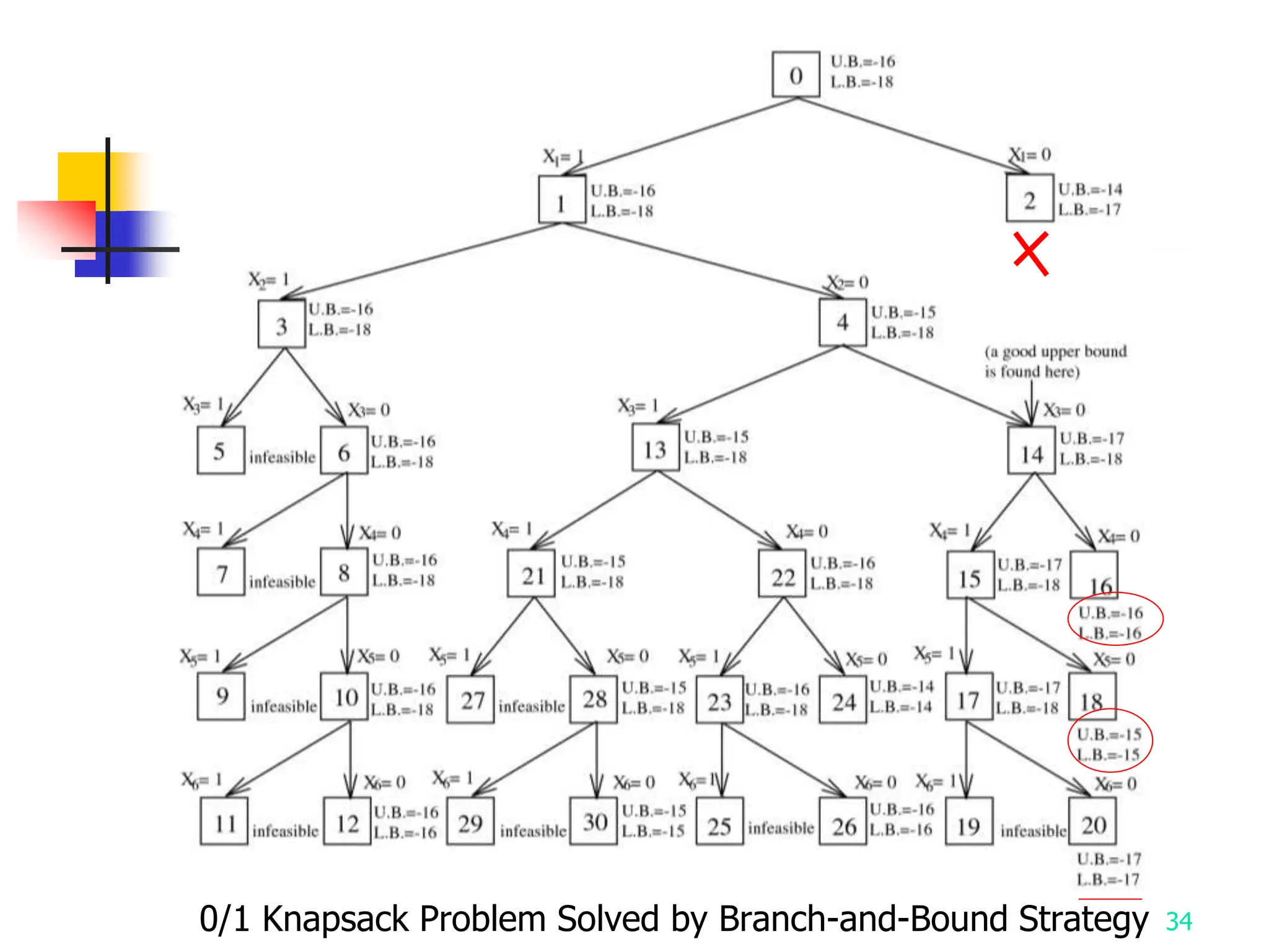
2) It describes applying branch and bound to the traveling salesman problem and 0/1 knapsack problem.
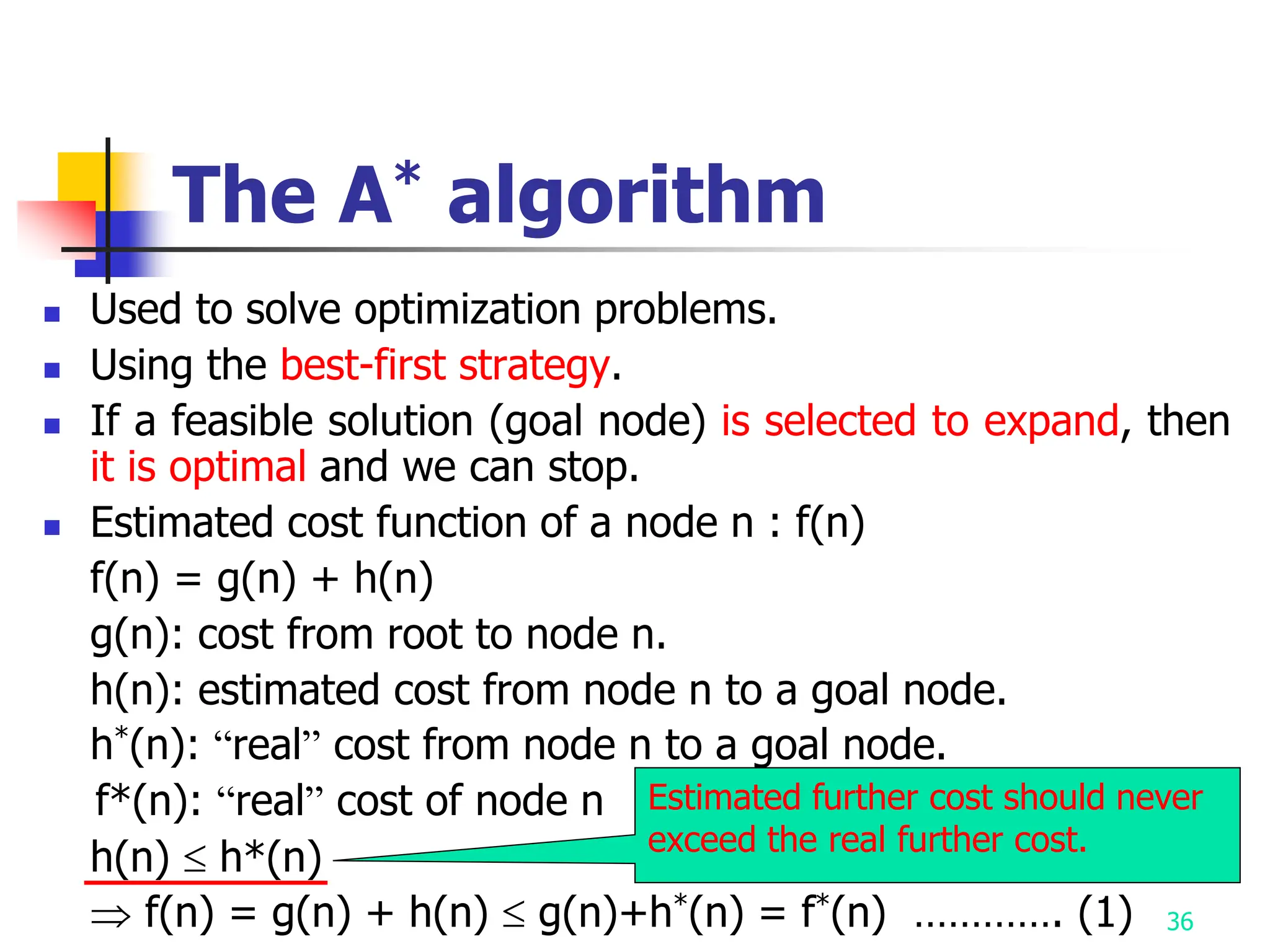
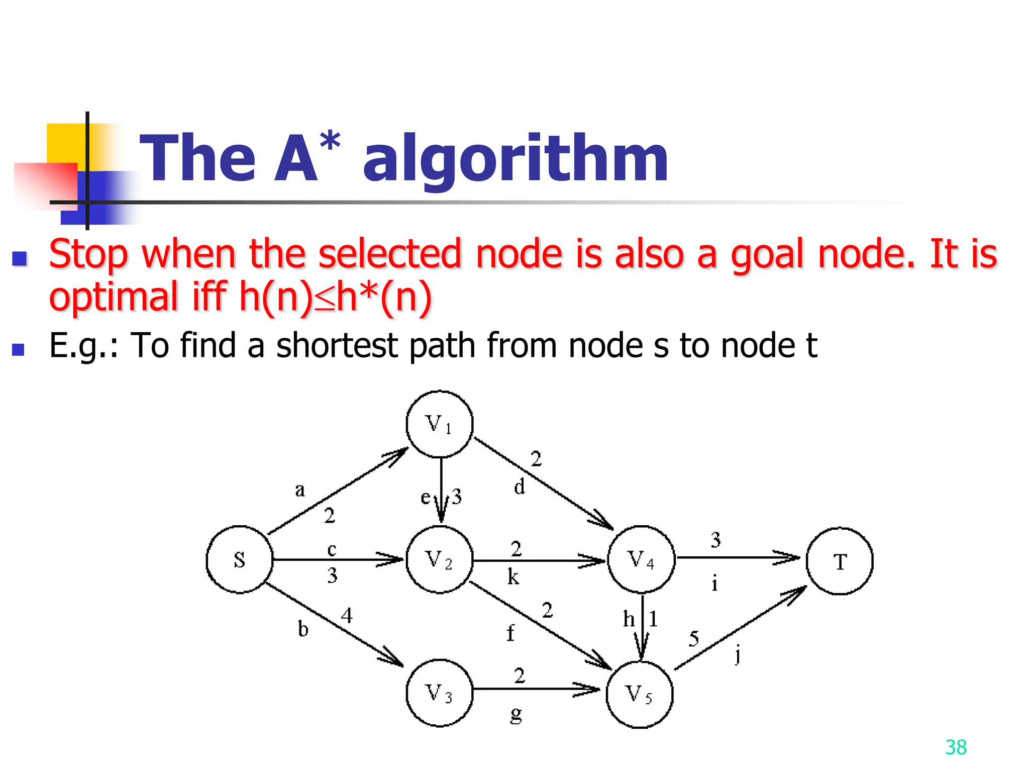
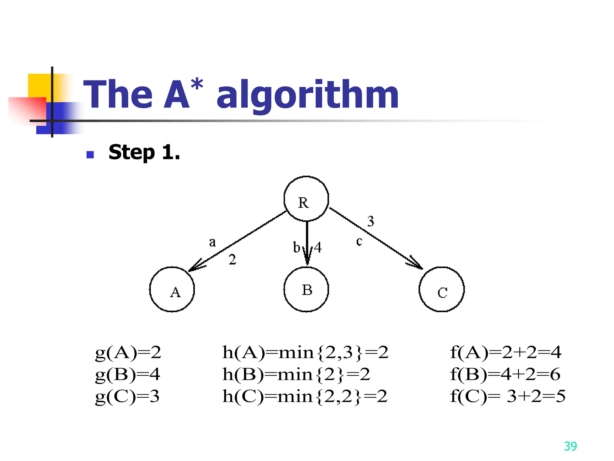
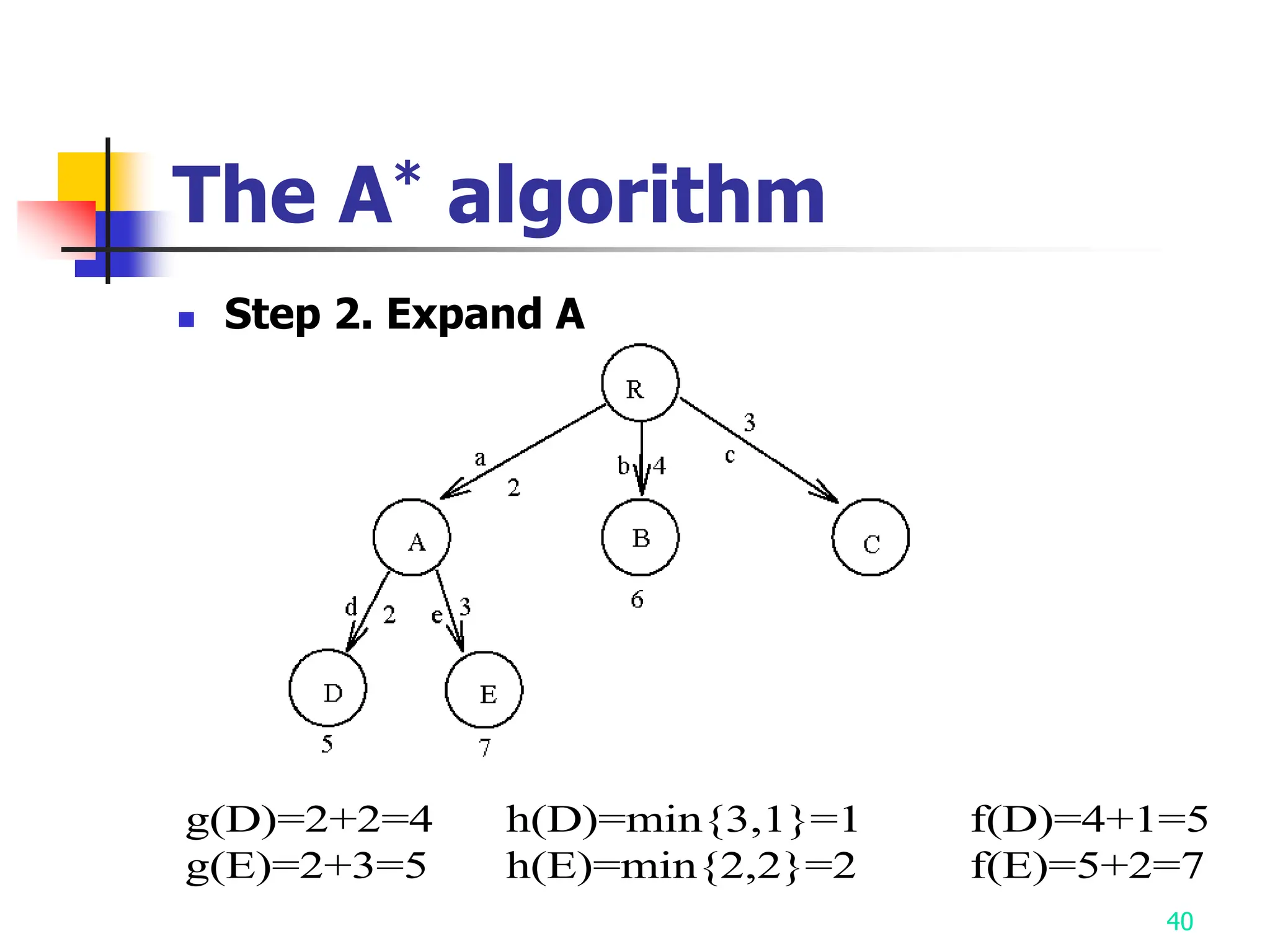
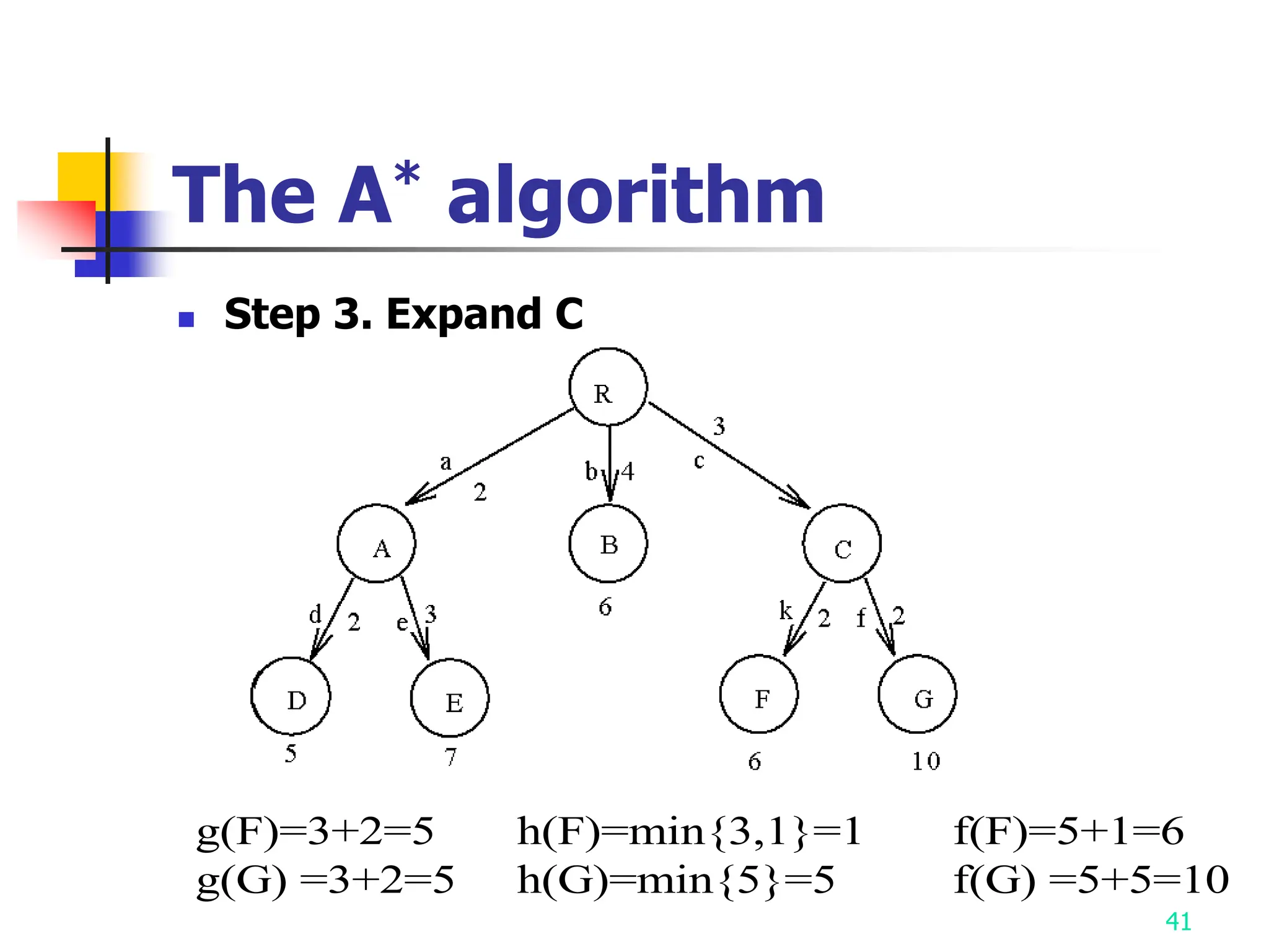
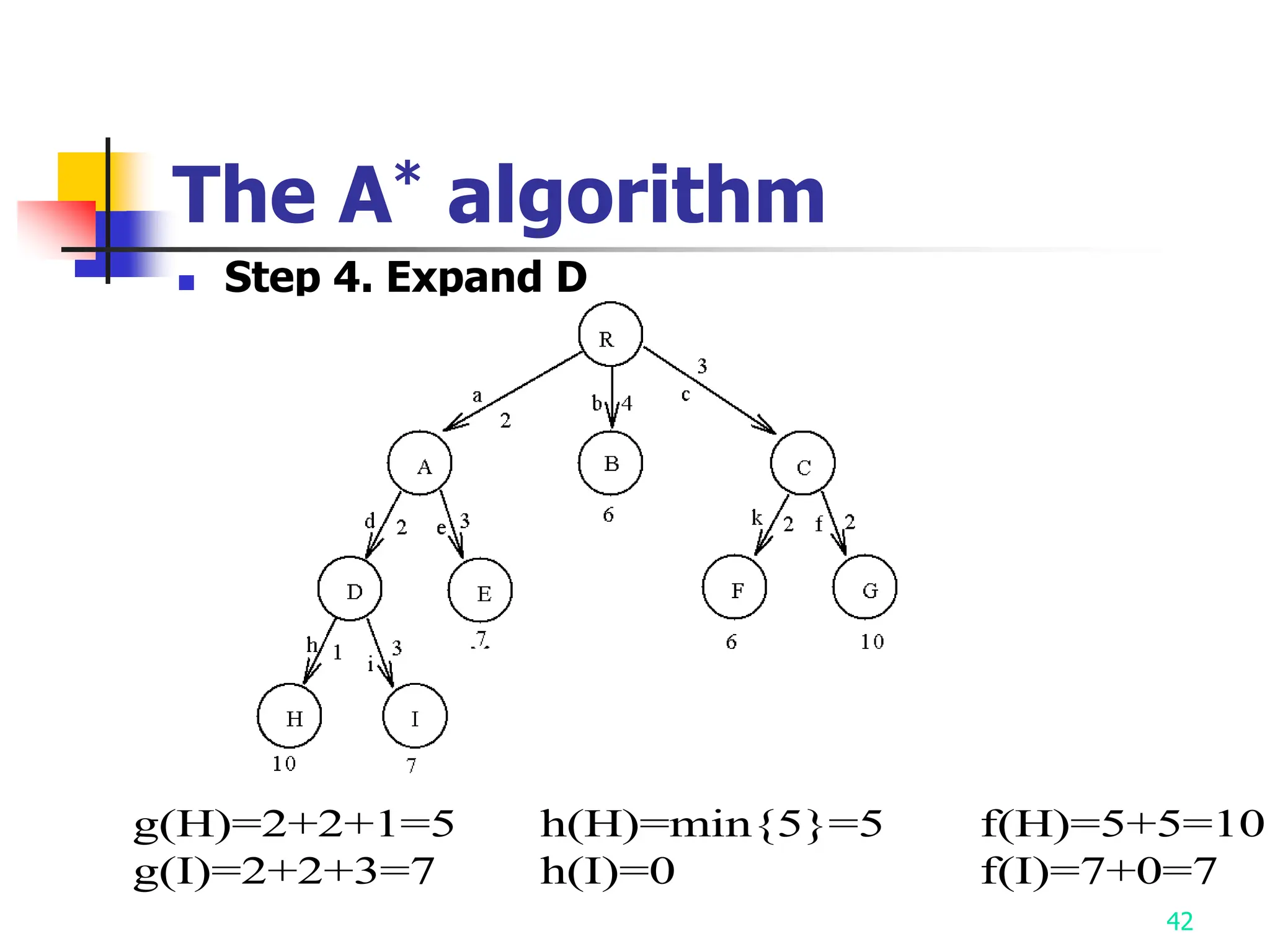
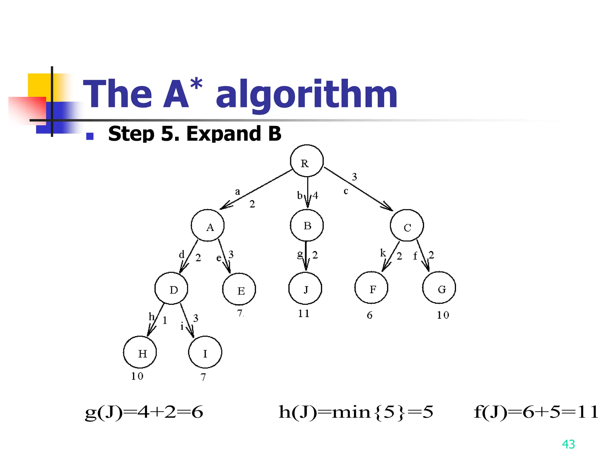
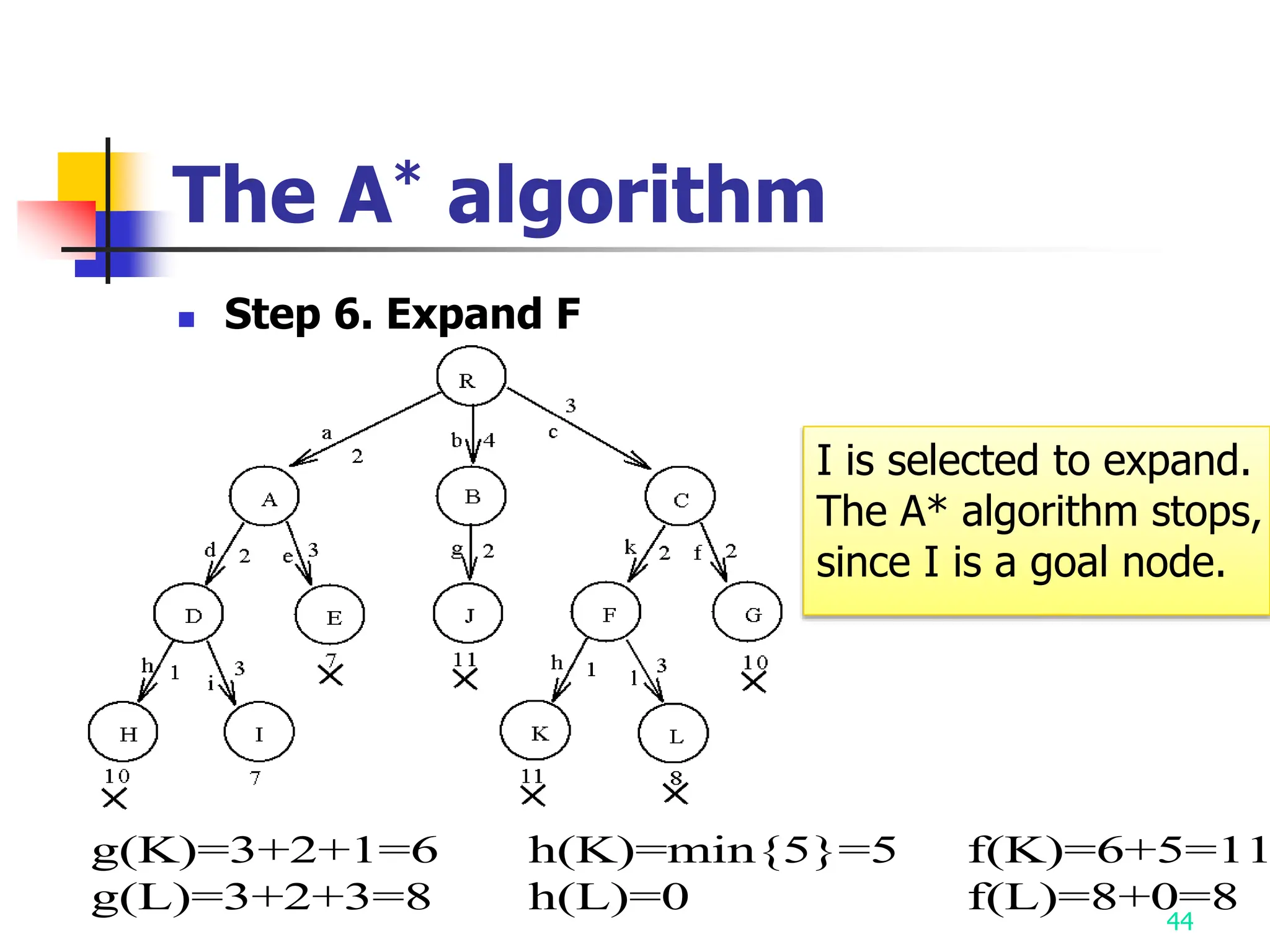
3) The A* algorithm is also discussed as it uses best-first search to find optimal solutions by estimating costs with heuristic functions.