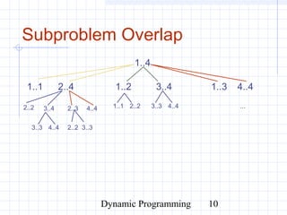
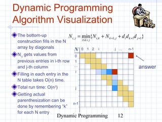
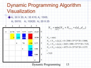
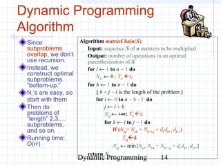
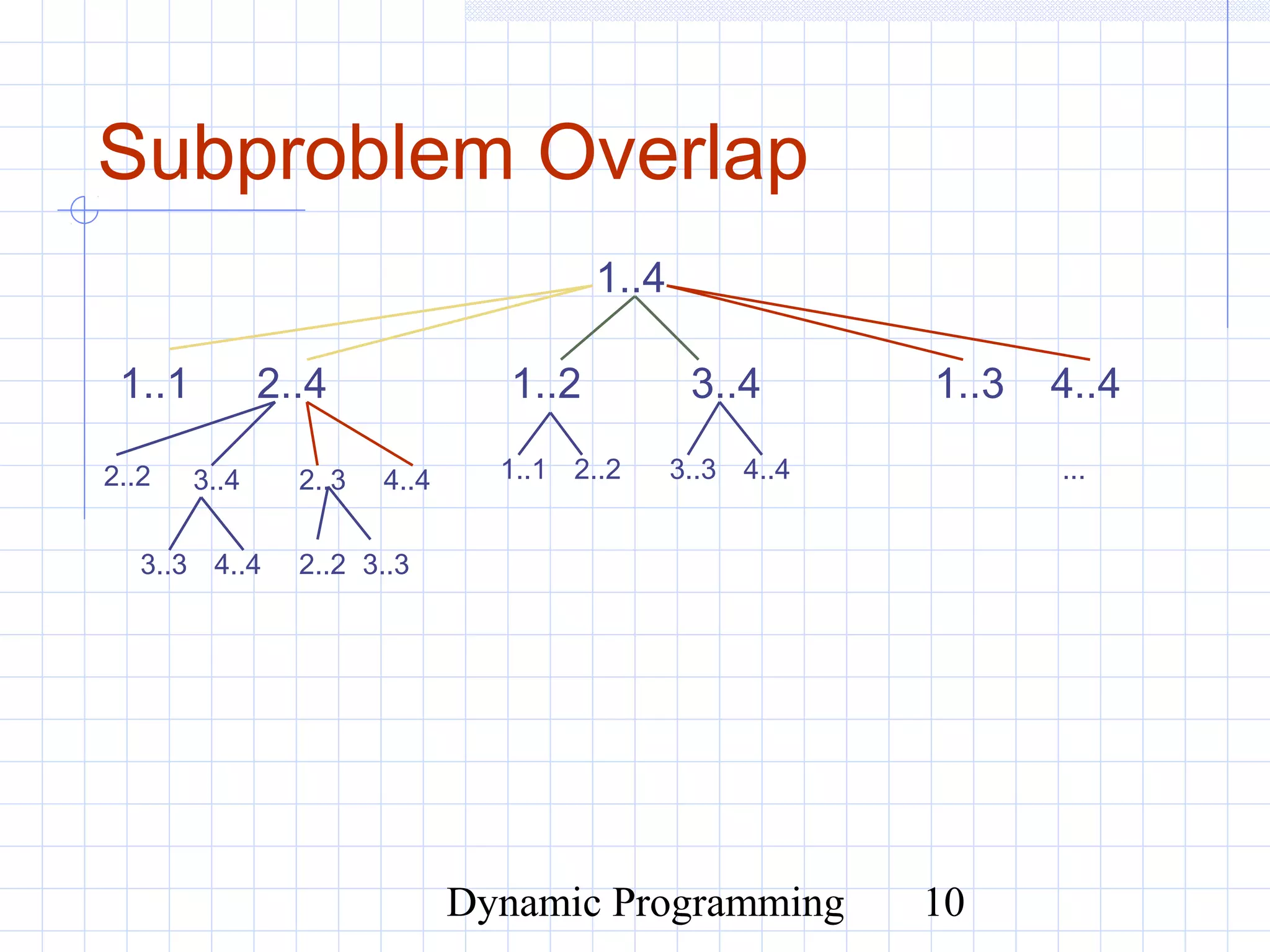
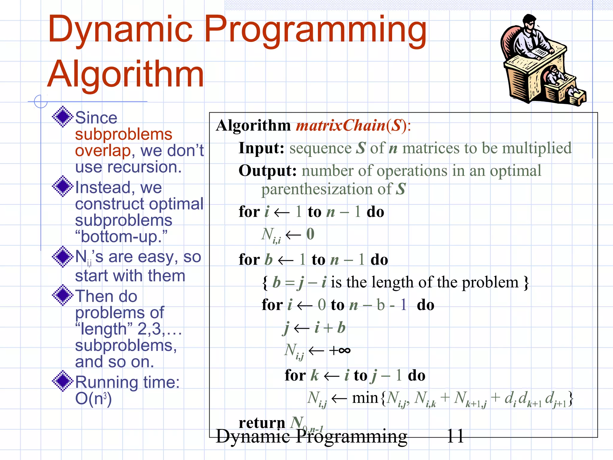
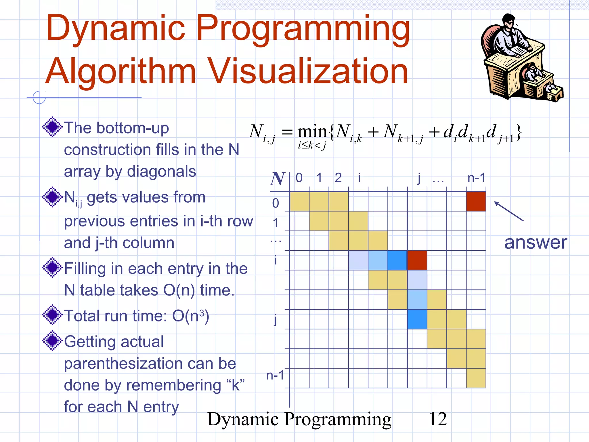
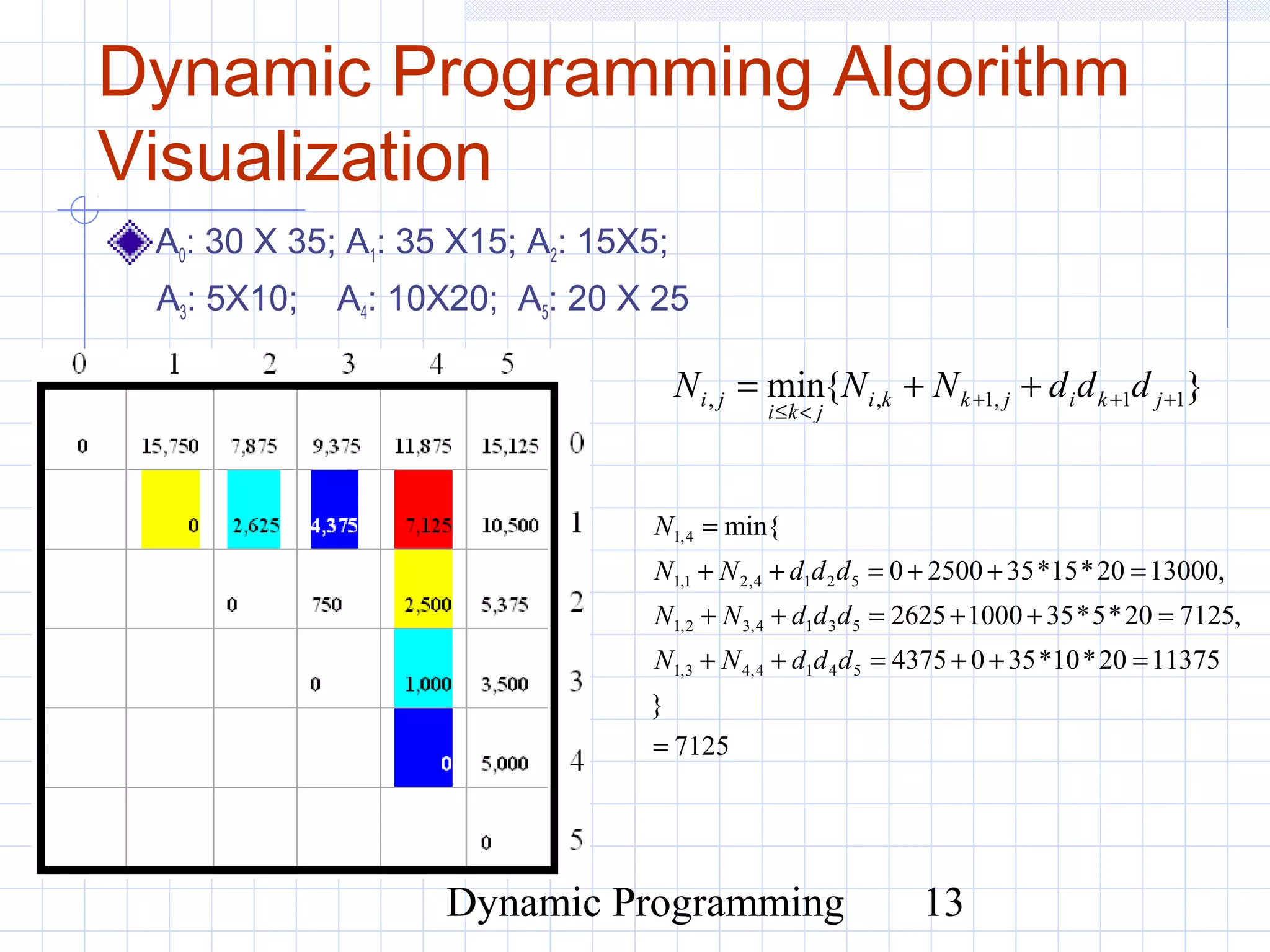
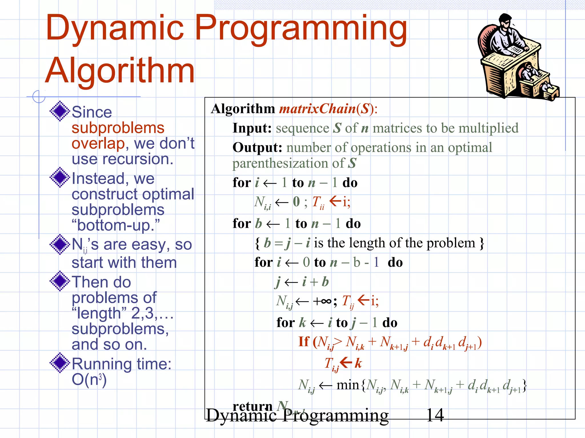
Dynamic programming is an algorithm design paradigm that can be applied to problems exhibiting optimal substructure and overlapping subproblems. It works by breaking down a problem into subproblems and storing the results of already solved subproblems, rather than recomputing them multiple times. This allows for an efficient bottom-up approach. Examples where dynamic programming can be applied include the matrix chain multiplication problem, the 0-1 knapsack problem, and finding the longest common subsequence between two strings.
![Dynamic Programming 3
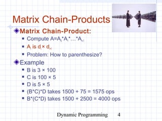
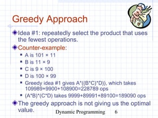
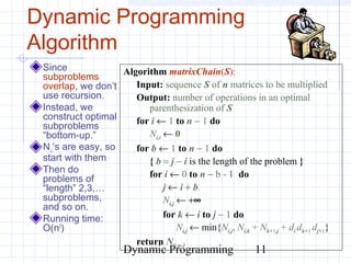
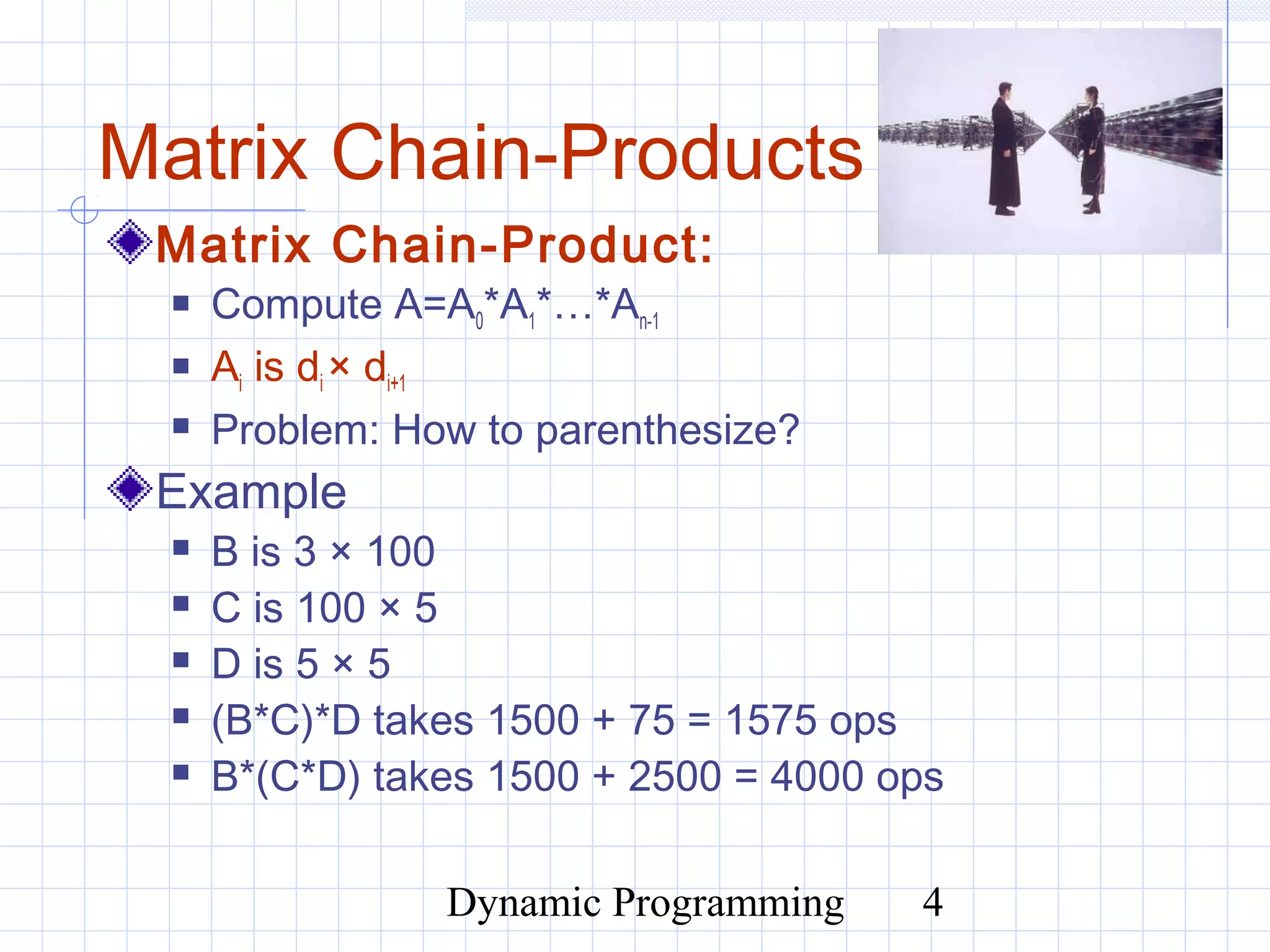
Matrix Chain-Products
Dynamic Programming is a general
algorithm design paradigm.
Rather than give the general structure, let
us first give a motivating example:
Matrix Chain-Products
Review: Matrix Multiplication.
C = A*B
A is d × e and B is e × f
O(d⋅e⋅f ) time
A C
B
d d
f
e
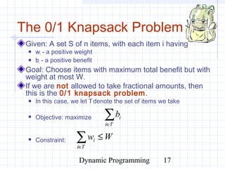
f
e
i
j
i,j
∑
−
=
=
1
0
],[*],[],[
e
k
jkBkiAjiC](https://image.slidesharecdn.com/5-150507111808-lva1-app6892/85/5-3-dynamic-programming-03-3-320.jpg)
![Dynamic Programming 19
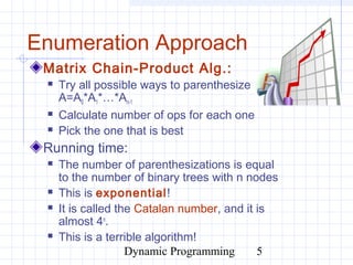
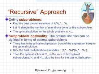
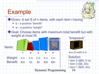
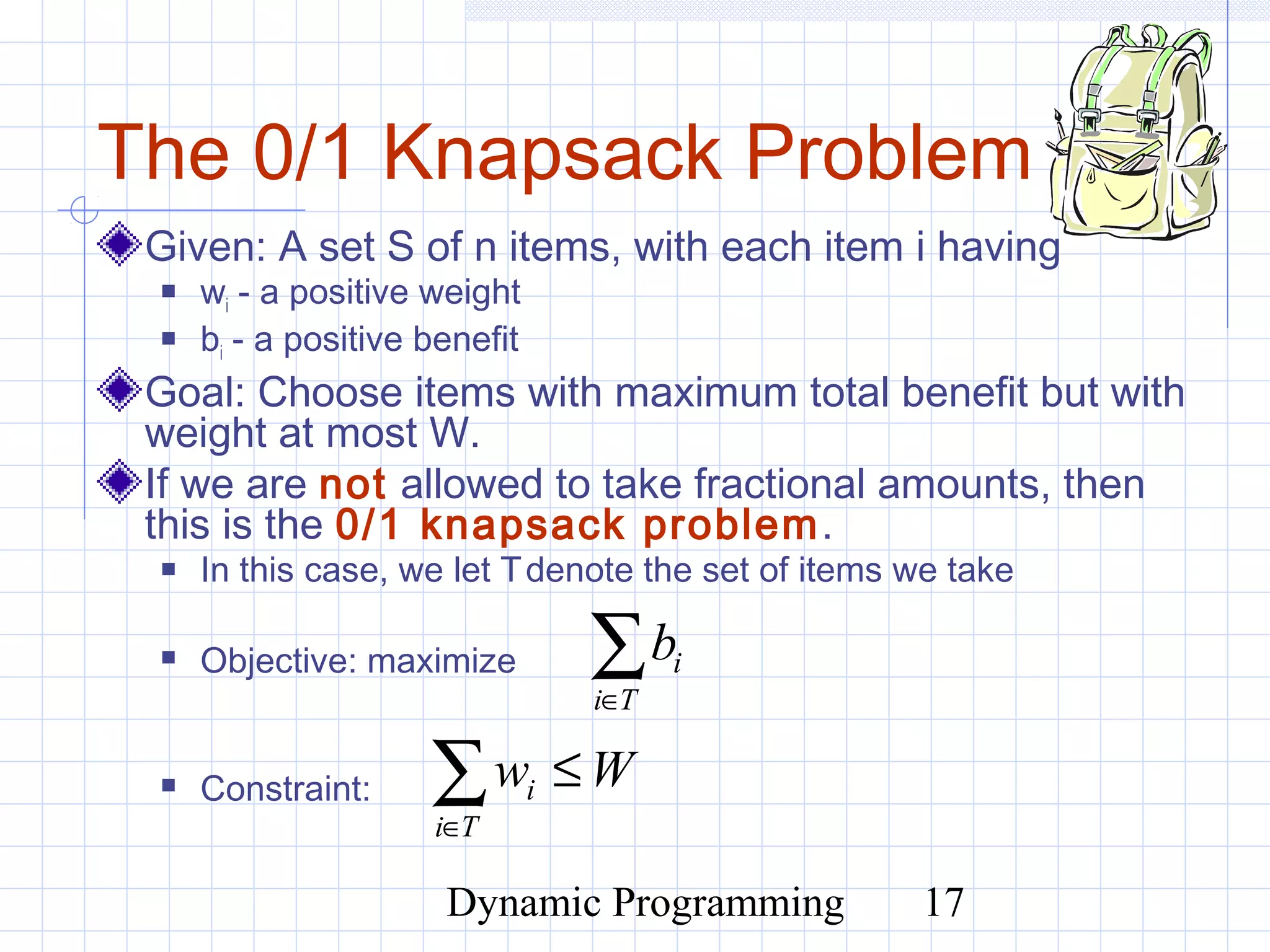
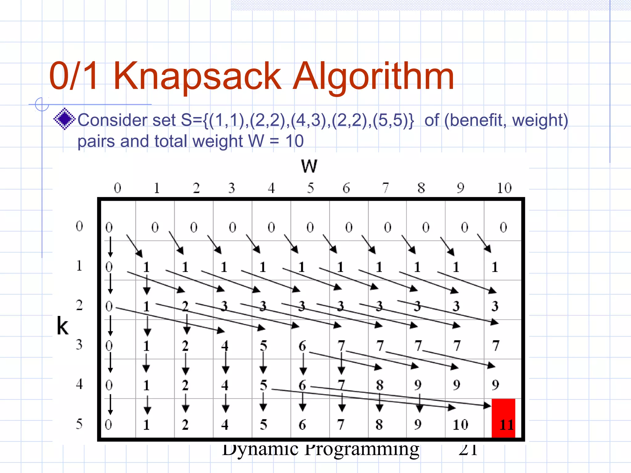
A 0/1 Knapsack Algorithm,
First Attempt
Sk: Set of items numbered 1 to k.
Define B[k] = best selection from Sk.
Problem: does not have subproblem optimality:
Consider set S={(3,2),(5,4),(8,5),(4,3),(10,9)} of
(benefit, weight) pairs and total weight W = 20
Best for S4:
Best for S5:](https://image.slidesharecdn.com/5-150507111808-lva1-app6892/85/5-3-dynamic-programming-03-19-320.jpg)
![Dynamic Programming 20
A 0/1 Knapsack Algorithm,
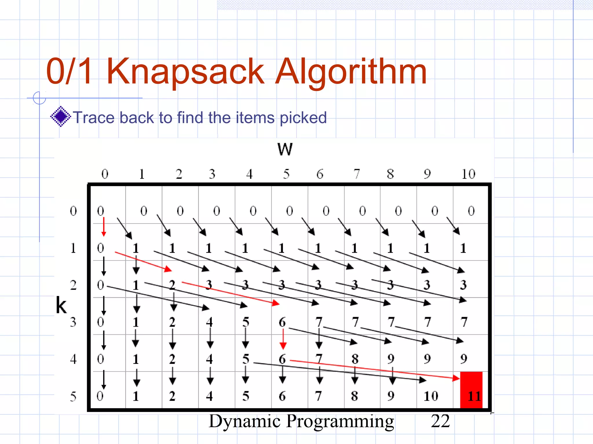
Second Attempt
Sk: Set of items numbered 1 to k.
Define B[k,w] to be the best selection from Sk with
weight at most w
Good news: this does have subproblem optimality.
I.e., the best subset of Sk with weight at most w is either
the best subset of Sk-1 with weight at most w or
the best subset of Sk-1 with weight at most w−wk plus item k
+−−−
>−
=
else}],1[],,1[max{
if],1[
],[
kk
k
bwwkBwkB
wwwkB
wkB](https://image.slidesharecdn.com/5-150507111808-lva1-app6892/85/5-3-dynamic-programming-03-20-320.jpg)
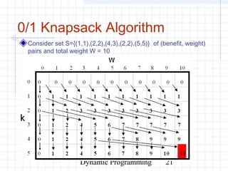
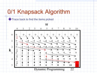
![Dynamic Programming 24
0/1 Knapsack Algorithm
Recall the definition of
B[k,w]
Since B[k,w] is defined in
terms of B[k−1,*], we can
use two arrays of instead of
a matrix
Running time: O(nW).
Not a polynomial-time
algorithm since W may be
large
This is a pseudo-polynomial
time algorithm
Algorithm 01Knapsack(S, W):
Input: set S of n items with benefit bi
and weight wi; maximum weight W
Output: benefit of best subset of S with
weight at most W
let A and B be arrays of length W + 1
for w ← 0 to W do
B[w] ← 0
for k ← 1 to n do
copy array B into array A
for w ← wk to W do
if A[w−wk] + bk > A[w] then
B[w] ← A[w−wk] + bk
return B[W]
+−−−
>−
=
else}],1[],,1[max{
if],1[
],[
kk
k
bwwkBwkB
wwwkB
wkB](https://image.slidesharecdn.com/5-150507111808-lva1-app6892/85/5-3-dynamic-programming-03-24-320.jpg)
![Dynamic Programming 28
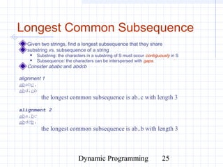
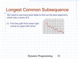
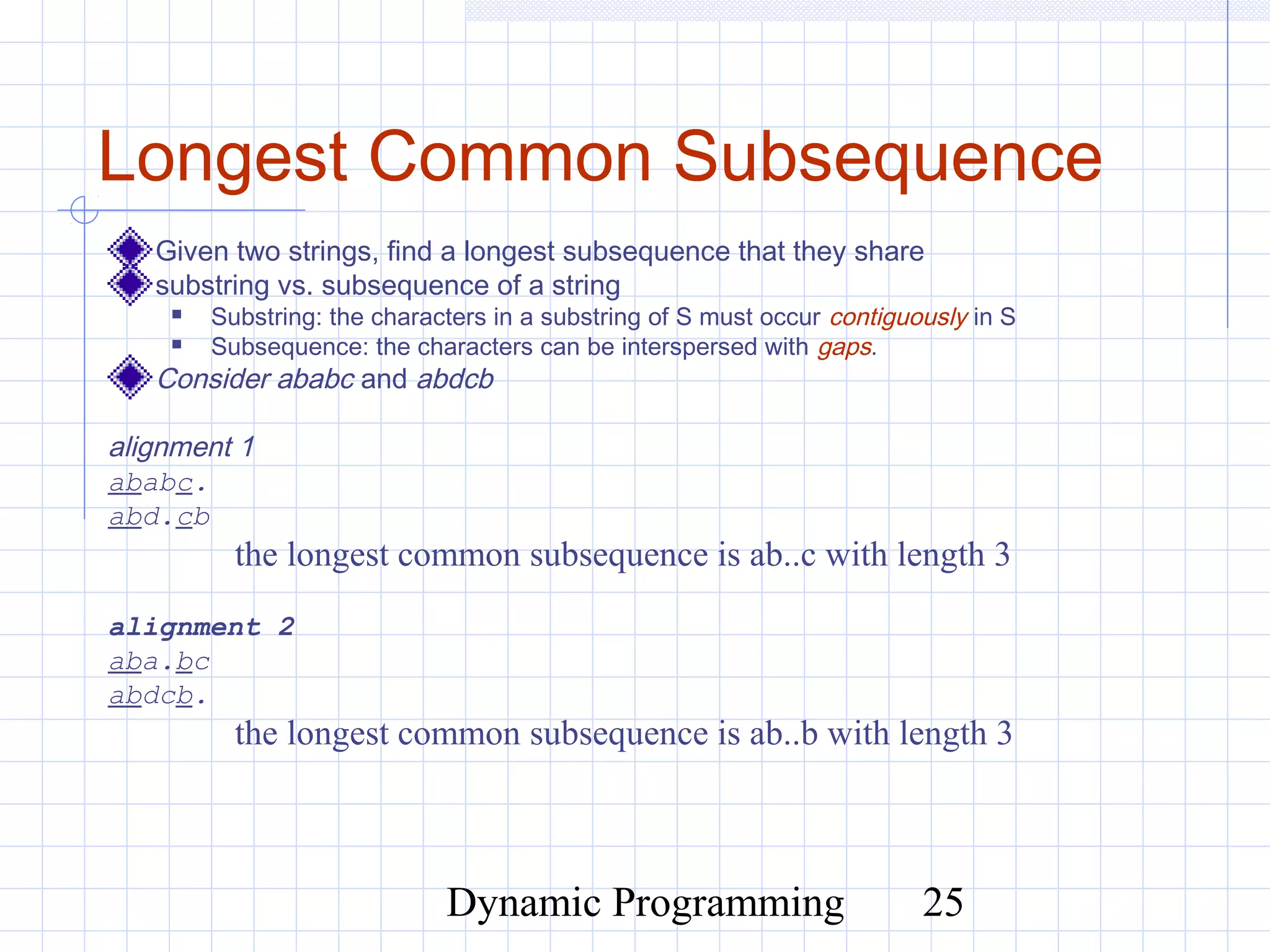
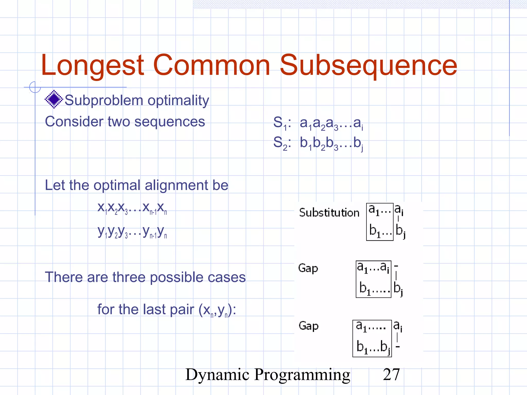
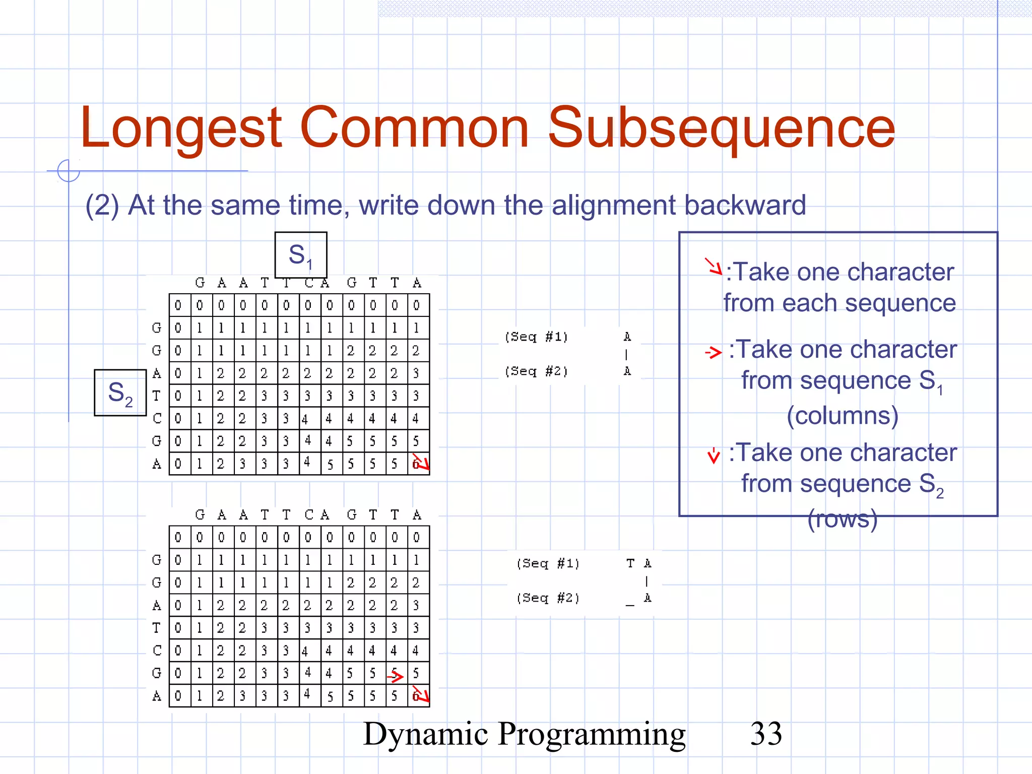
Longest Common Subsequence
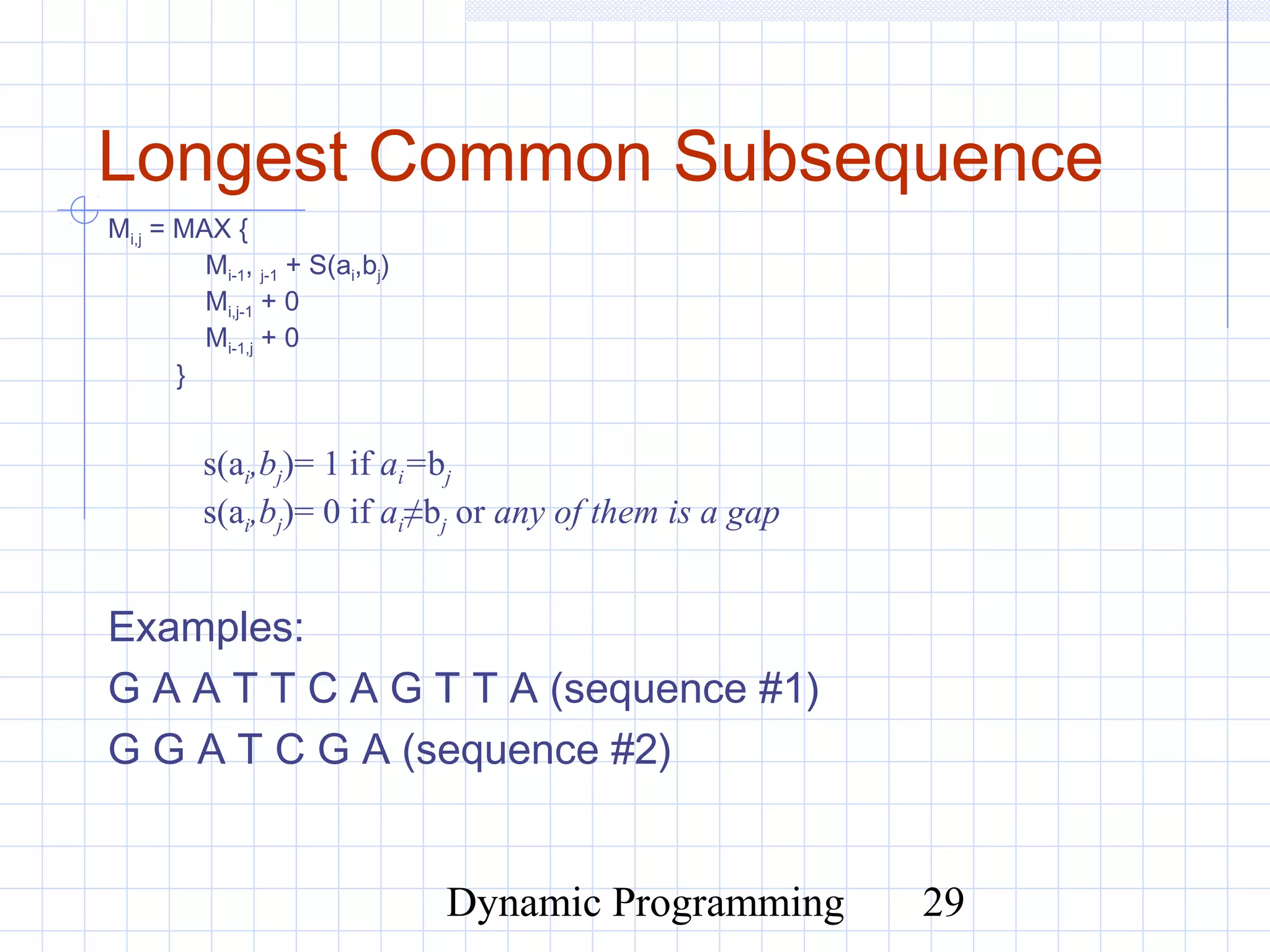
Mi,j = MAX {Mi-1, j-1 + S (ai,bj) (match/mismatch)
Mi,j-1 + 0 (gap in sequence #1)
Mi-1,j + 0 (gap in sequence #2) }
Mi,jis the score for optimal alignment between strings a[1…i] (substring of
a from index 1 to i) and b[1…j]
S1: a1a2a3…ai
S2: b1b2b3…bj
There are three cases for (xn,yn) pair:
x1x2x3…xn-1xn
y1y2y3…yn-1yn](https://image.slidesharecdn.com/5-150507111808-lva1-app6892/85/5-3-dynamic-programming-03-28-320.jpg)
![Dynamic Programming 30
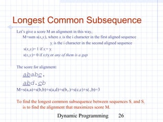
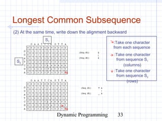
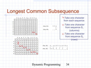
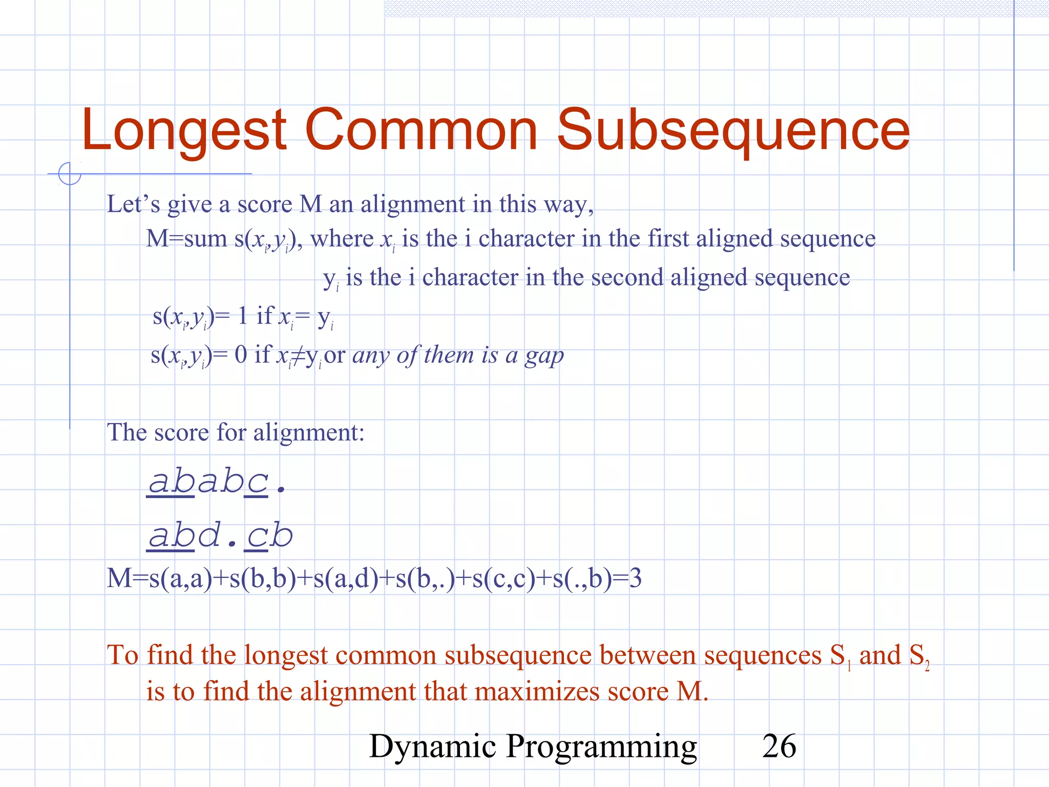
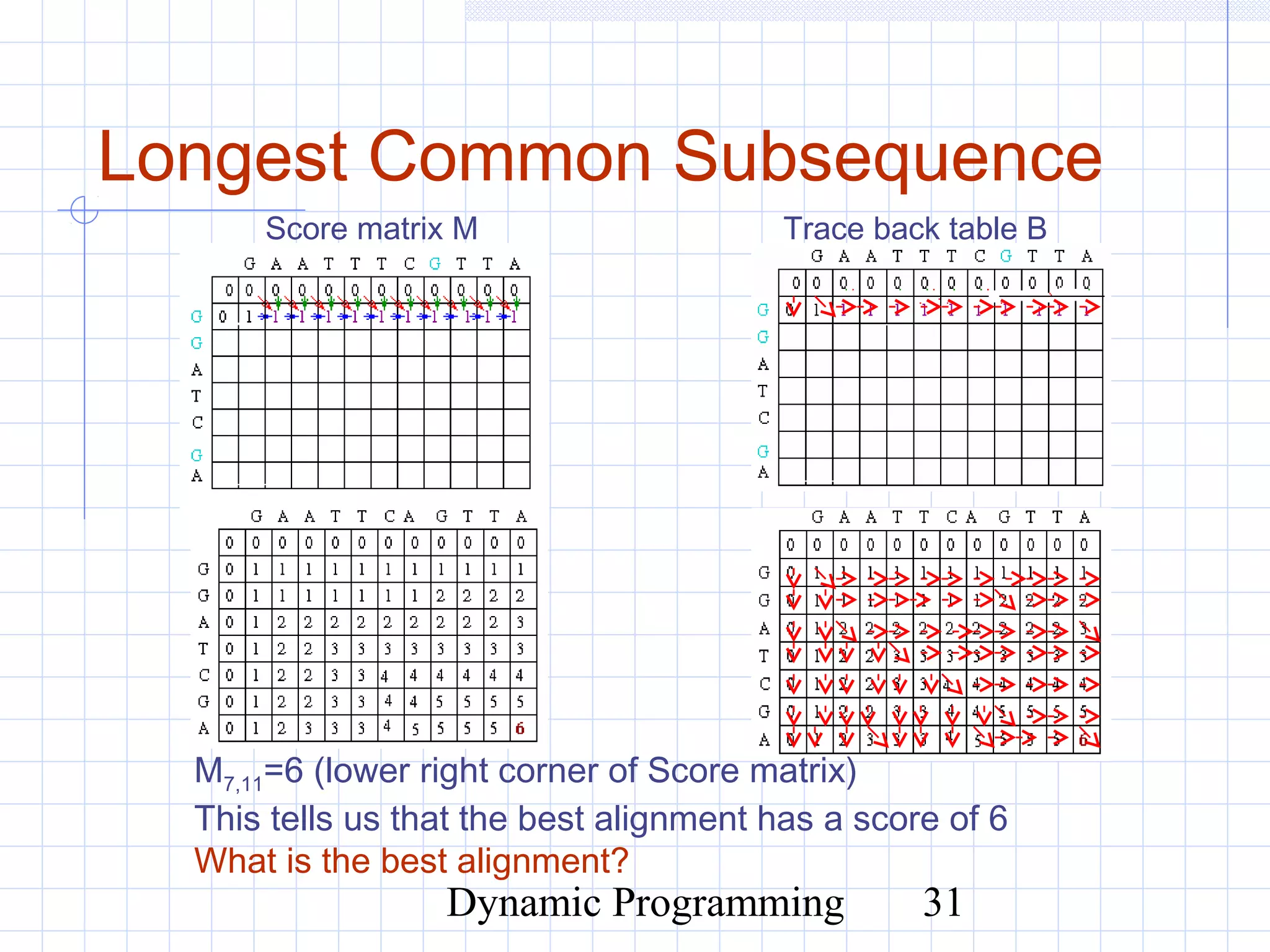
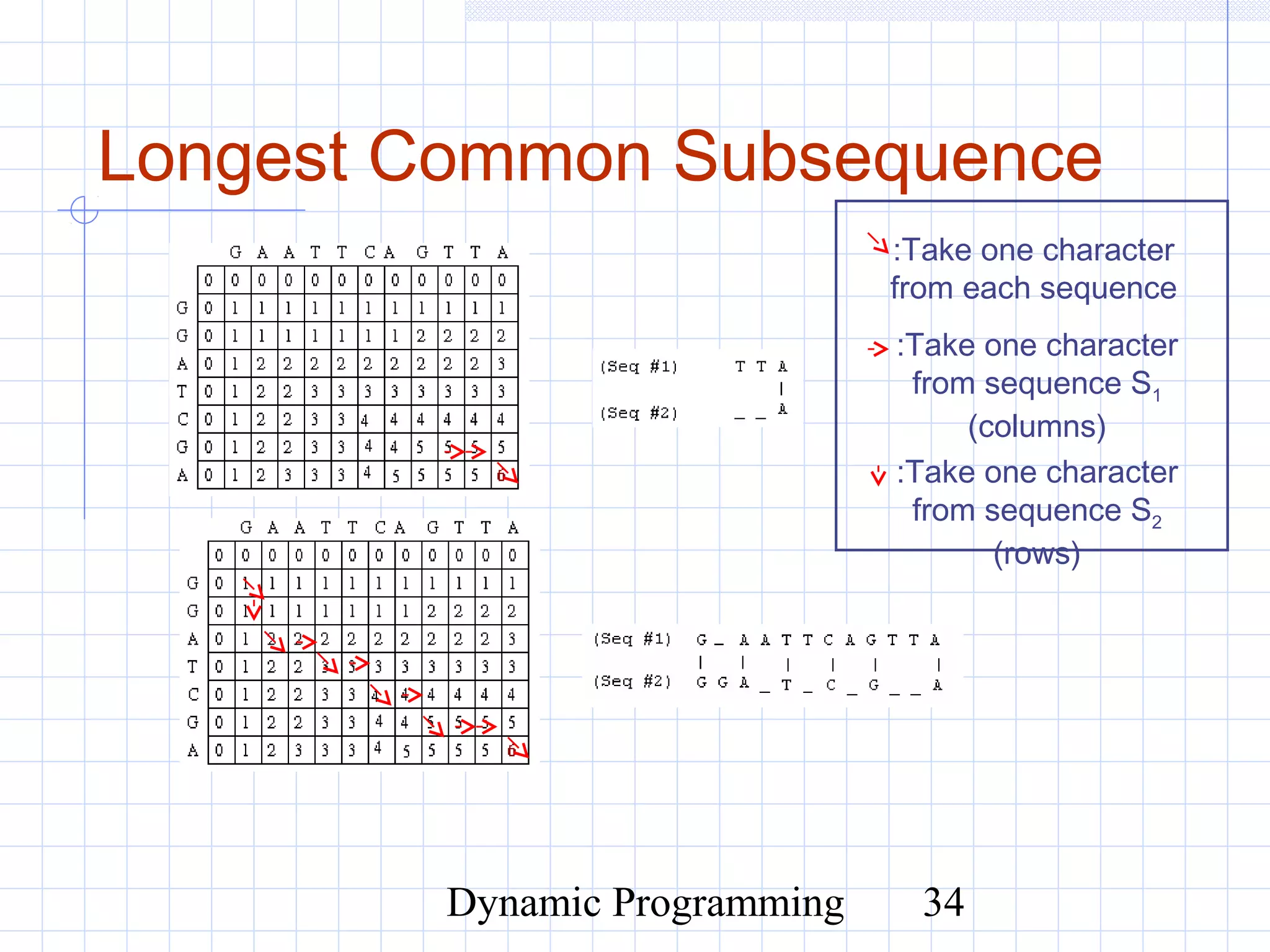
Longest Common Subsequence
M1,1 = MAX[M0,0 + 1, M1, 0 + 0, M0,1 + 0] = MAX [1, 0, 0] = 1
Fill the score matrix M and trace back table B
Score matrix M Trace back table B](https://image.slidesharecdn.com/5-150507111808-lva1-app6892/85/5-3-dynamic-programming-03-30-320.jpg)

![Dynamic Programming 36
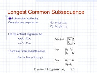
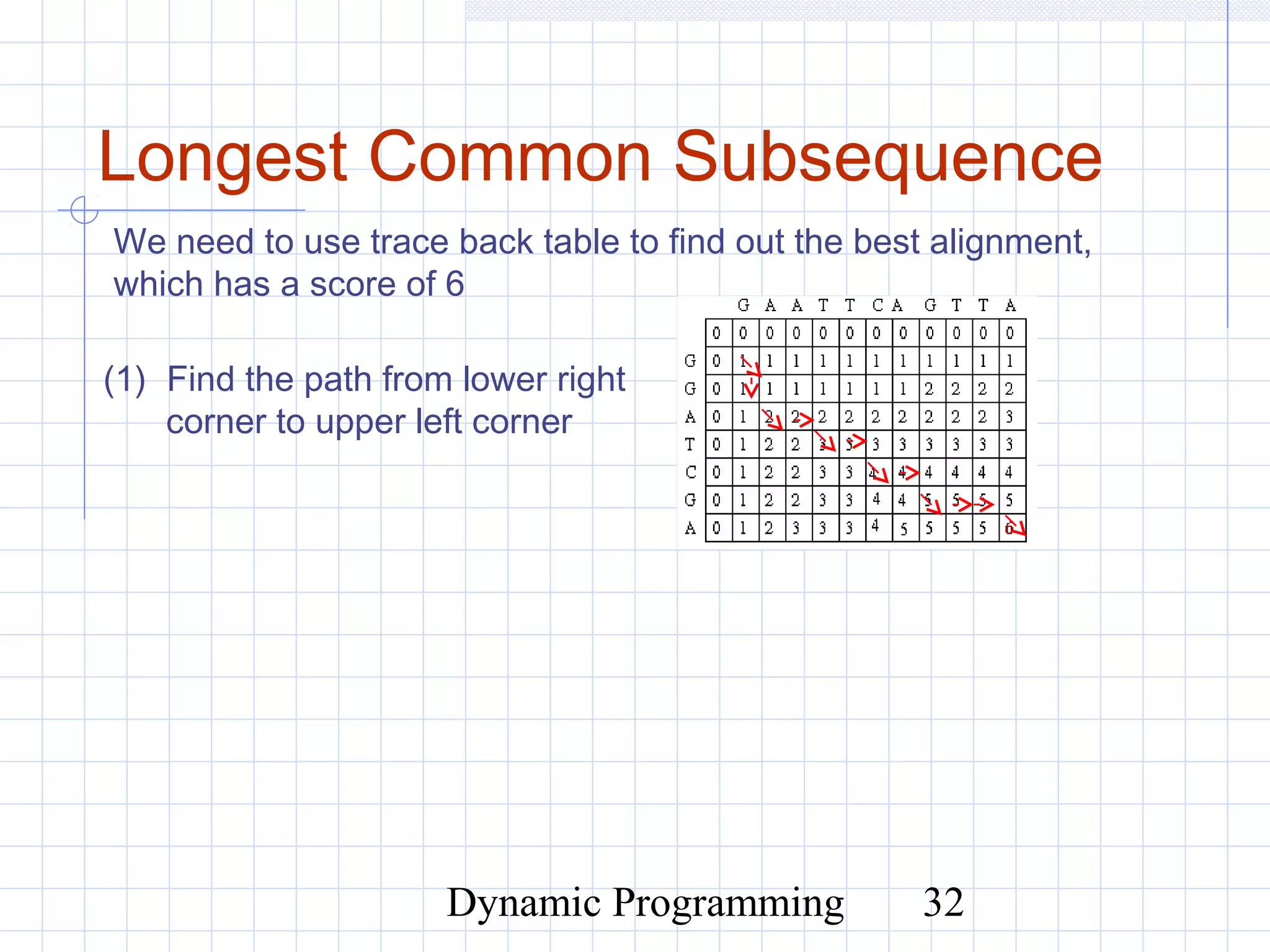
Longest Common Subsequence
Algorithm LCS (string A, string B) {
Input strings A and B
Output the longest common subsequence of A and B
M: Score Matrix
B: trace back table (use letter a, b, c for )
n=A.length()
m=B.length()
// fill in M and B
for (i=0;i<m+1;i++)
for (j=0;j<n+1;j++)
if (i==0) || (j==0)
then M(i,j)=0;
else if (A[i]==B[j])
M(i,j)=max {M[i-1,j-1]+1, M[i-1,j], M[i,j-1]}
{update the entry in trace table B}
else
M(i,j)=max {M[i-1,j-1], M[i-1,j], M[i,j-1]}
{update the entry in trace table B}
then use trace back table B to print out the optimal alignment
…](https://image.slidesharecdn.com/5-150507111808-lva1-app6892/85/5-3-dynamic-programming-03-36-320.jpg)
![Dynamic Programming 3
Matrix Chain-Products
Dynamic Programming is a general
algorithm design paradigm.
Rather than give the general structure, let
us first give a motivating example:
Matrix Chain-Products
Review: Matrix Multiplication.
C = A*B
A is d × e and B is e × f
O(d⋅e⋅f ) time
A C
B
d d
f
e
f
e
i
j
i,j
∑
−
=
=
1
0
],[*],[],[
e
k
jkBkiAjiC](https://image.slidesharecdn.com/5-150507111808-lva1-app6892/75/5-3-dynamic-programming-03-3-2048.jpg)

![Dynamic Programming 19
A 0/1 Knapsack Algorithm,
First Attempt
Sk: Set of items numbered 1 to k.
Define B[k] = best selection from Sk.
Problem: does not have subproblem optimality:
Consider set S={(3,2),(5,4),(8,5),(4,3),(10,9)} of
(benefit, weight) pairs and total weight W = 20
Best for S4:
Best for S5:](https://image.slidesharecdn.com/5-150507111808-lva1-app6892/75/5-3-dynamic-programming-03-19-2048.jpg)
![Dynamic Programming 20
A 0/1 Knapsack Algorithm,
Second Attempt
Sk: Set of items numbered 1 to k.
Define B[k,w] to be the best selection from Sk with
weight at most w
Good news: this does have subproblem optimality.
I.e., the best subset of Sk with weight at most w is either
the best subset of Sk-1 with weight at most w or
the best subset of Sk-1 with weight at most w−wk plus item k
+−−−
>−
=
else}],1[],,1[max{
if],1[
],[
kk
k
bwwkBwkB
wwwkB
wkB](https://image.slidesharecdn.com/5-150507111808-lva1-app6892/75/5-3-dynamic-programming-03-20-2048.jpg)

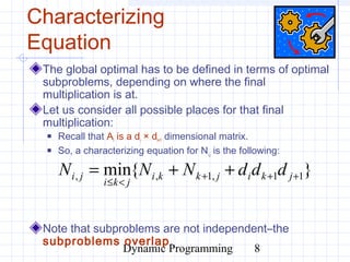
![Dynamic Programming 24
0/1 Knapsack Algorithm
Recall the definition of
B[k,w]
Since B[k,w] is defined in
terms of B[k−1,*], we can
use two arrays of instead of
a matrix
Running time: O(nW).
Not a polynomial-time
algorithm since W may be
large
This is a pseudo-polynomial
time algorithm
Algorithm 01Knapsack(S, W):
Input: set S of n items with benefit bi
and weight wi; maximum weight W
Output: benefit of best subset of S with
weight at most W
let A and B be arrays of length W + 1
for w ← 0 to W do
B[w] ← 0
for k ← 1 to n do
copy array B into array A
for w ← wk to W do
if A[w−wk] + bk > A[w] then
B[w] ← A[w−wk] + bk
return B[W]
+−−−
>−
=
else}],1[],,1[max{
if],1[
],[
kk
k
bwwkBwkB
wwwkB
wkB](https://image.slidesharecdn.com/5-150507111808-lva1-app6892/75/5-3-dynamic-programming-03-24-2048.jpg)
![Dynamic Programming 28
Longest Common Subsequence
Mi,j = MAX {Mi-1, j-1 + S (ai,bj) (match/mismatch)
Mi,j-1 + 0 (gap in sequence #1)
Mi-1,j + 0 (gap in sequence #2) }
Mi,jis the score for optimal alignment between strings a[1…i] (substring of
a from index 1 to i) and b[1…j]
S1: a1a2a3…ai
S2: b1b2b3…bj
There are three cases for (xn,yn) pair:
x1x2x3…xn-1xn
y1y2y3…yn-1yn](https://image.slidesharecdn.com/5-150507111808-lva1-app6892/75/5-3-dynamic-programming-03-28-2048.jpg)
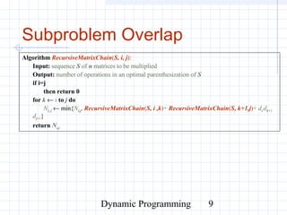
![Dynamic Programming 30
Longest Common Subsequence
M1,1 = MAX[M0,0 + 1, M1, 0 + 0, M0,1 + 0] = MAX [1, 0, 0] = 1
Fill the score matrix M and trace back table B
Score matrix M Trace back table B](https://image.slidesharecdn.com/5-150507111808-lva1-app6892/75/5-3-dynamic-programming-03-30-2048.jpg)
![Dynamic Programming 36
Longest Common Subsequence
Algorithm LCS (string A, string B) {
Input strings A and B
Output the longest common subsequence of A and B
M: Score Matrix
B: trace back table (use letter a, b, c for )
n=A.length()
m=B.length()
// fill in M and B
for (i=0;i<m+1;i++)
for (j=0;j<n+1;j++)
if (i==0) || (j==0)
then M(i,j)=0;
else if (A[i]==B[j])
M(i,j)=max {M[i-1,j-1]+1, M[i-1,j], M[i,j-1]}
{update the entry in trace table B}
else
M(i,j)=max {M[i-1,j-1], M[i-1,j], M[i,j-1]}
{update the entry in trace table B}
then use trace back table B to print out the optimal alignment
…](https://image.slidesharecdn.com/5-150507111808-lva1-app6892/75/5-3-dynamic-programming-03-36-2048.jpg)


![평범한 이야기[Intro: 2015 의기제]](https://cdn.slidesharecdn.com/ss_thumbnails/1stcardslide-150505225911-conversion-gate02-thumbnail.jpg?width=600ounds&width=560&fit=bounds)


