Downloaded 13 times


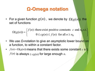
![Machine-independent time: An example
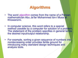
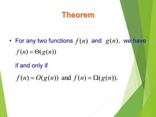
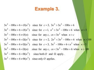
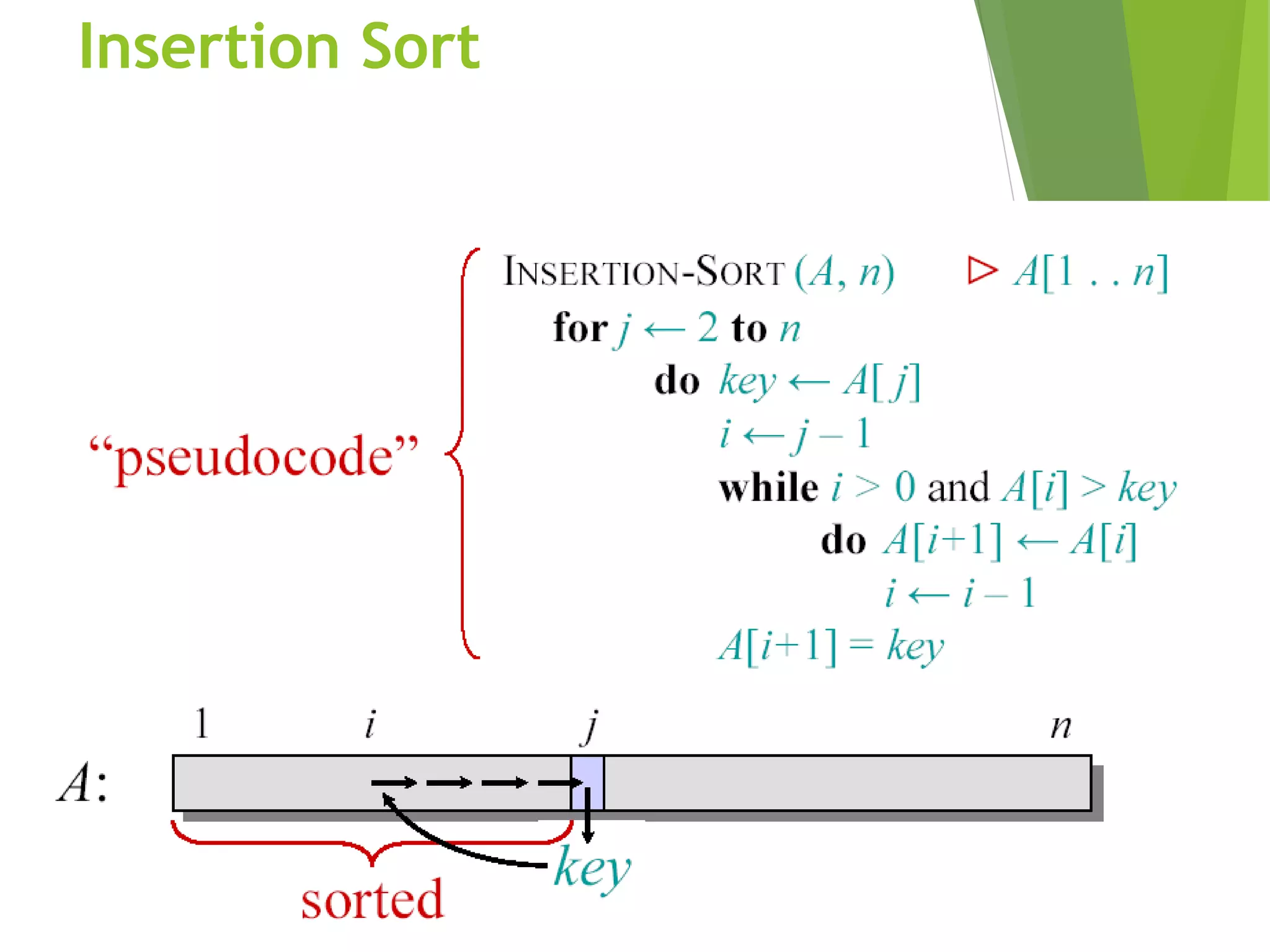
A pseudocode for insertion sort ( INSERTION SORT ).
INSERTION-SORT(A)
1 for j 2 to length [A]
2 do key A[ j]
3 Insert A[j] into the sortted sequence A[1,..., j-1].
4 i j – 1
5 while i > 0 and A[i] > key
6 do A[i+1] A[i]
7 i i – 1
8 A[i +1] key](https://image.slidesharecdn.com/algorithm-201217183802/85/Algorithm-in-Computer-Sorting-and-Notations-23-320.jpg)
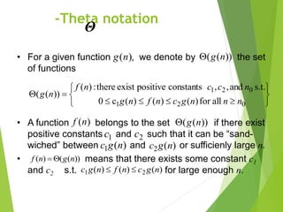
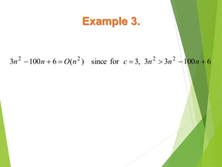
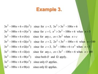
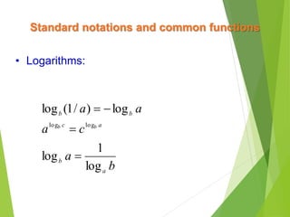
![Analysis of INSERTION-SORT(contd.)
1]1[8
)1(17
)1(][]1[6
][05
114
10]11[sequence
sortedtheinto][Insert3
1][2
][21
timescostSORT(A)-INSERTION
8
27
26
25
4
2
1
nckeyiA
tcii
tciAiA
tckeyiAandi
ncji
njA
jA
ncjAkey
ncAlengthj
n
j j
n
j j
n
j j
do
while
do
tofor](https://image.slidesharecdn.com/algorithm-201217183802/85/Algorithm-in-Computer-Sorting-and-Notations-24-320.jpg)


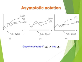


![Machine-independent time: An example
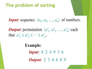
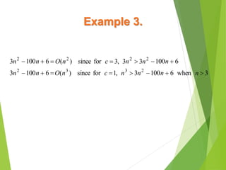
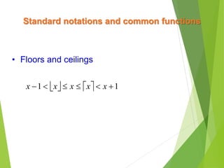
A pseudocode for insertion sort ( INSERTION SORT ).
INSERTION-SORT(A)
1 for j 2 to length [A]
2 do key A[ j]
3 Insert A[j] into the sortted sequence A[1,..., j-1].
4 i j – 1
5 while i > 0 and A[i] > key
6 do A[i+1] A[i]
7 i i – 1
8 A[i +1] key](https://image.slidesharecdn.com/algorithm-201217183802/75/Algorithm-in-Computer-Sorting-and-Notations-23-2048.jpg)
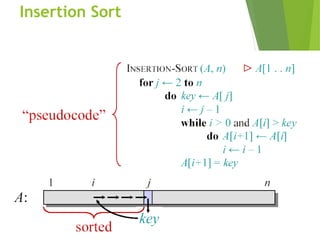
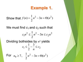
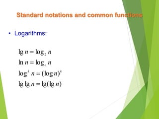
![Analysis of INSERTION-SORT(contd.)
1]1[8
)1(17
)1(][]1[6
][05
114
10]11[sequence
sortedtheinto][Insert3
1][2
][21
timescostSORT(A)-INSERTION
8
27
26
25
4
2
1
nckeyiA
tcii
tciAiA
tckeyiAandi
ncji
njA
jA
ncjAkey
ncAlengthj
n
j j
n
j j
n
j j
do
while
do
tofor](https://image.slidesharecdn.com/algorithm-201217183802/75/Algorithm-in-Computer-Sorting-and-Notations-24-2048.jpg)
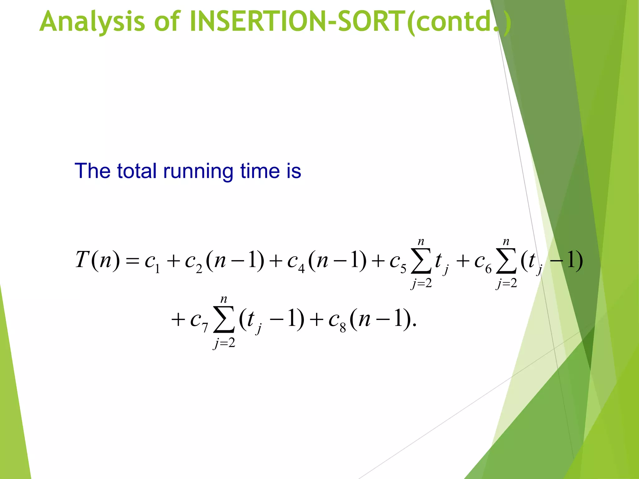

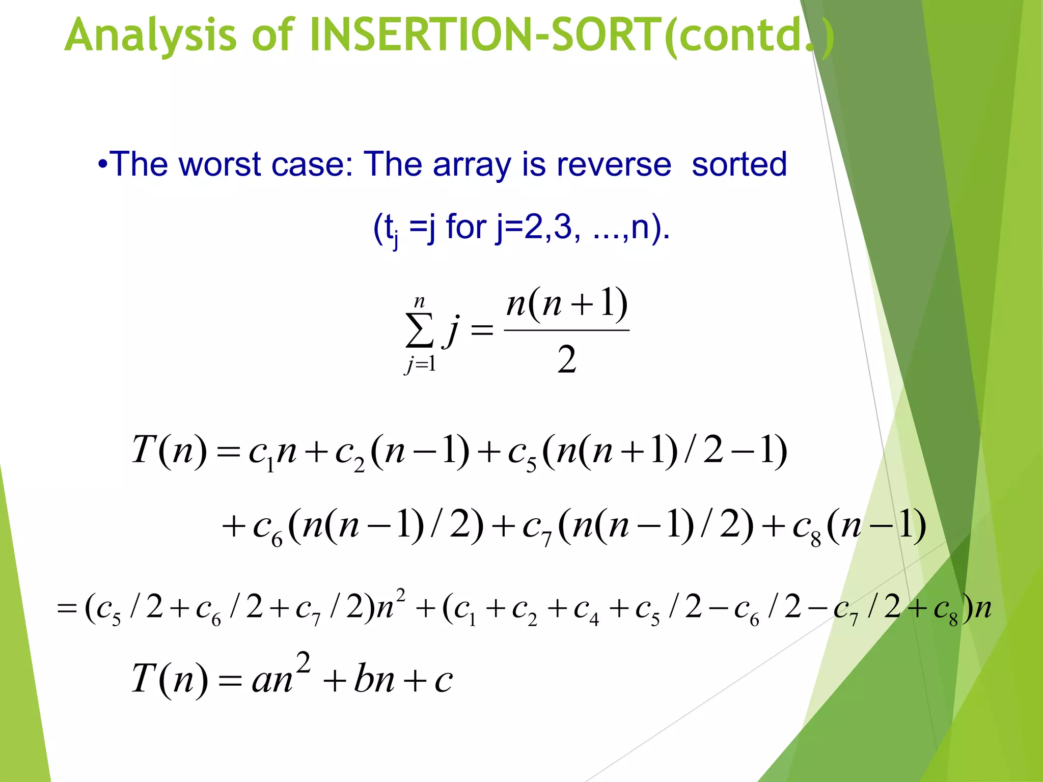
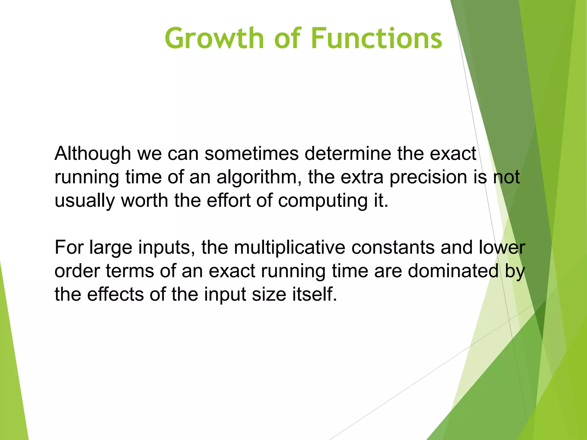
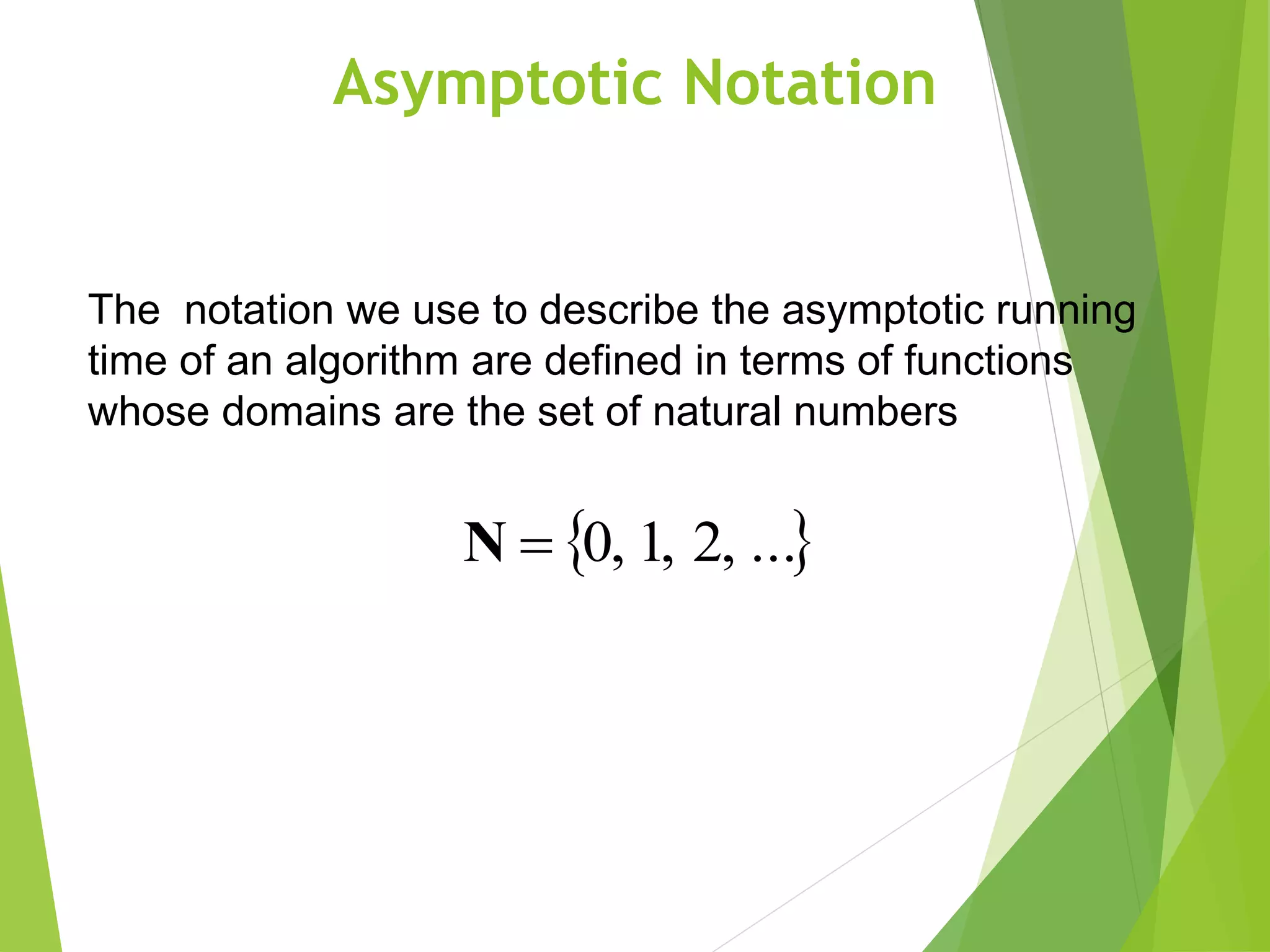
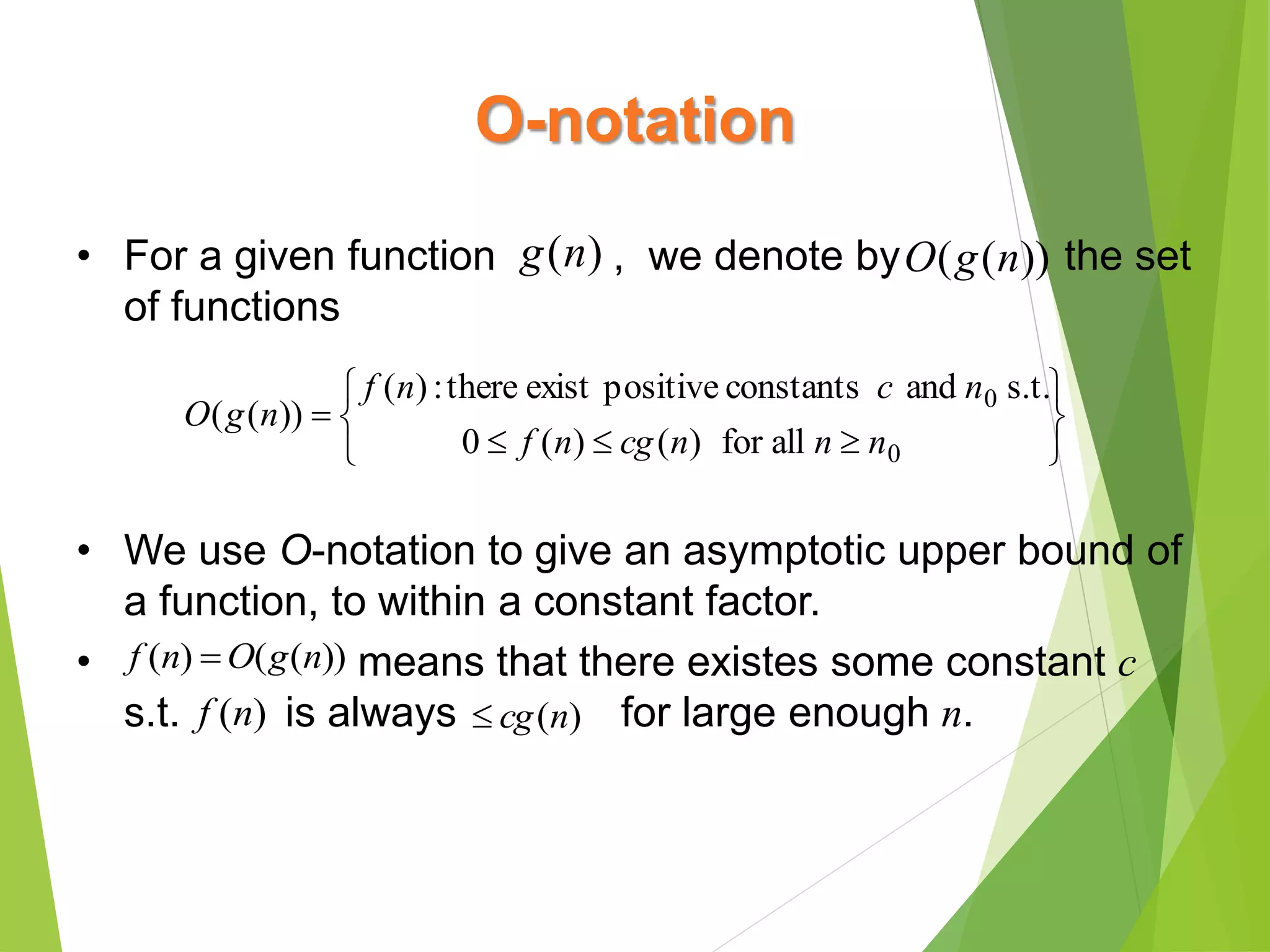
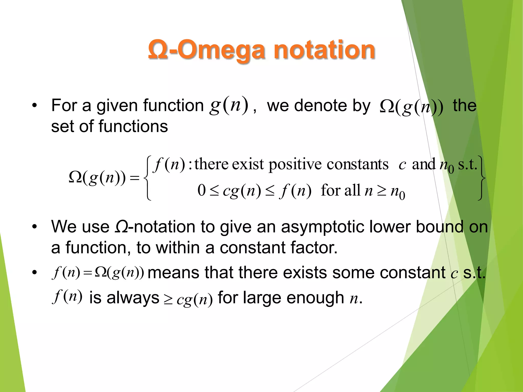
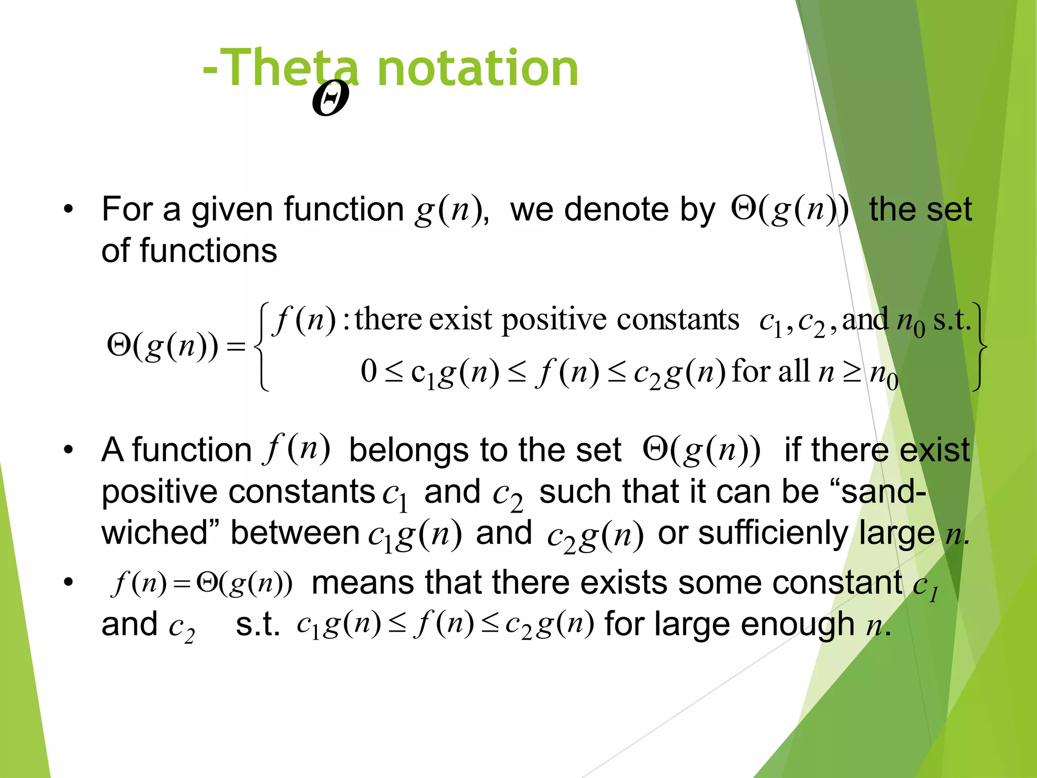
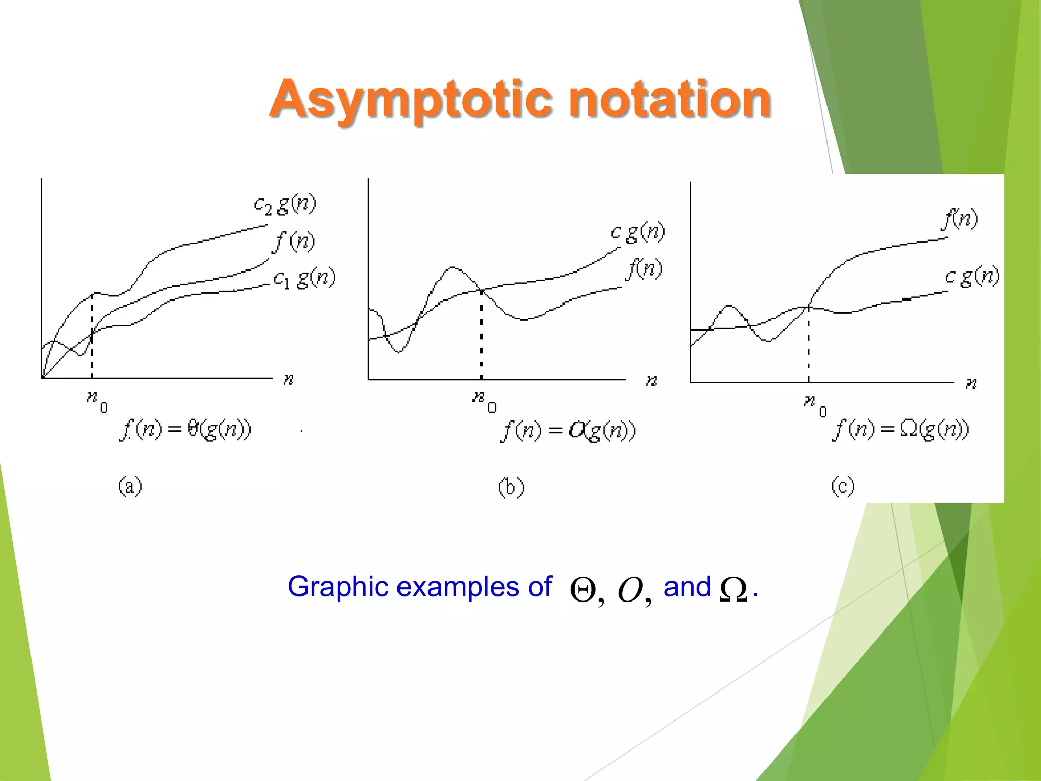
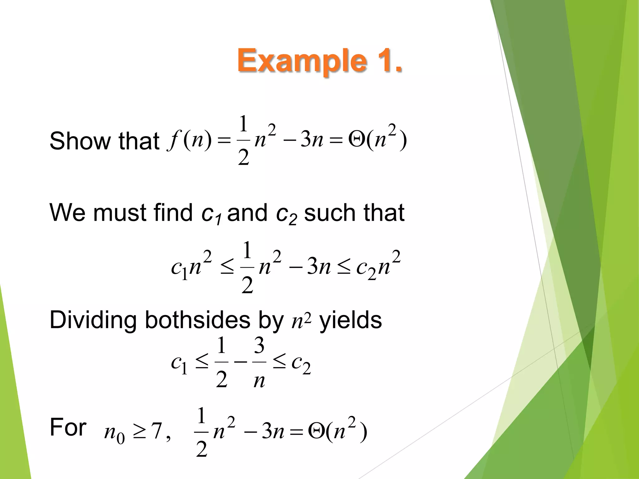
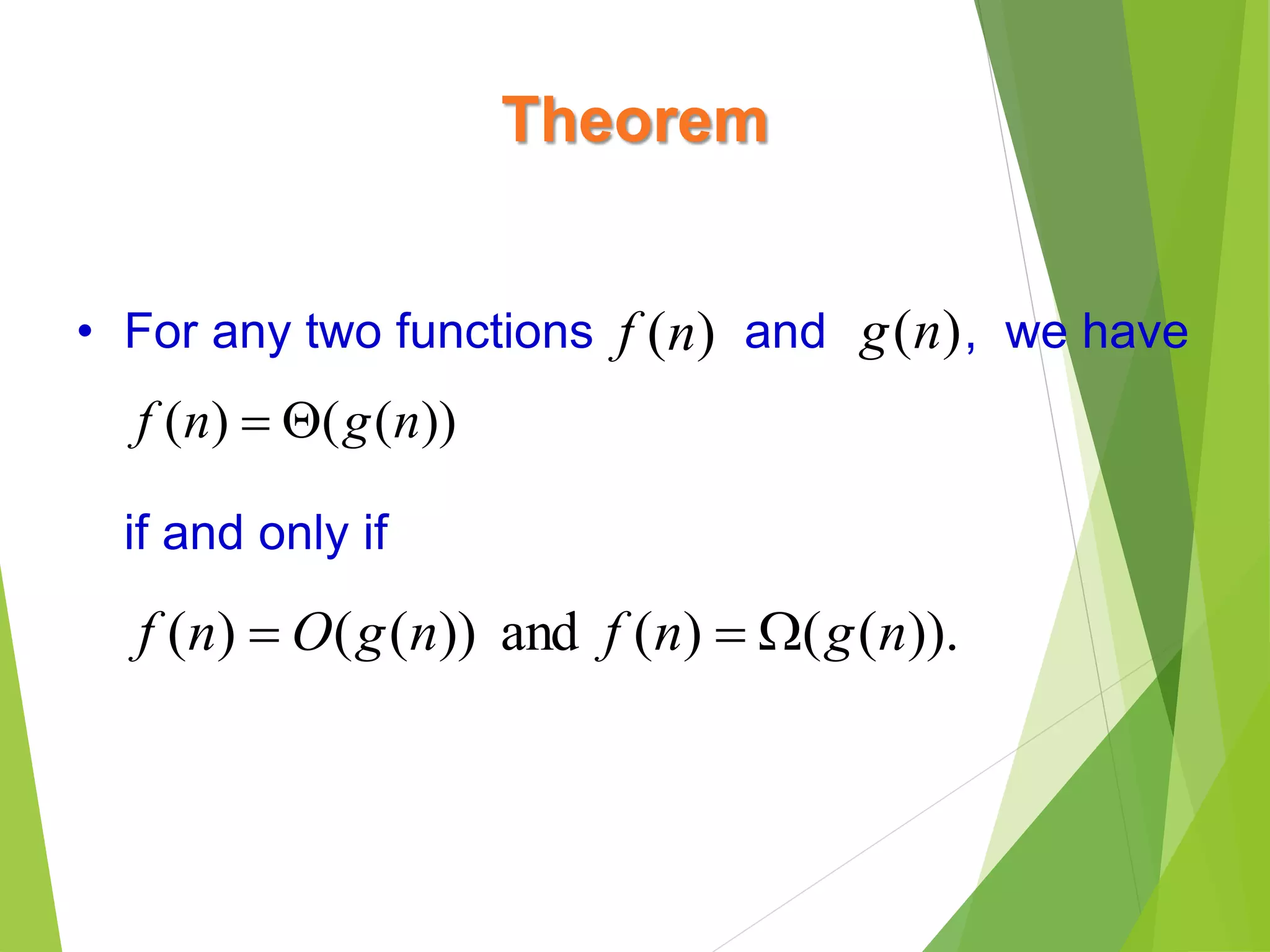
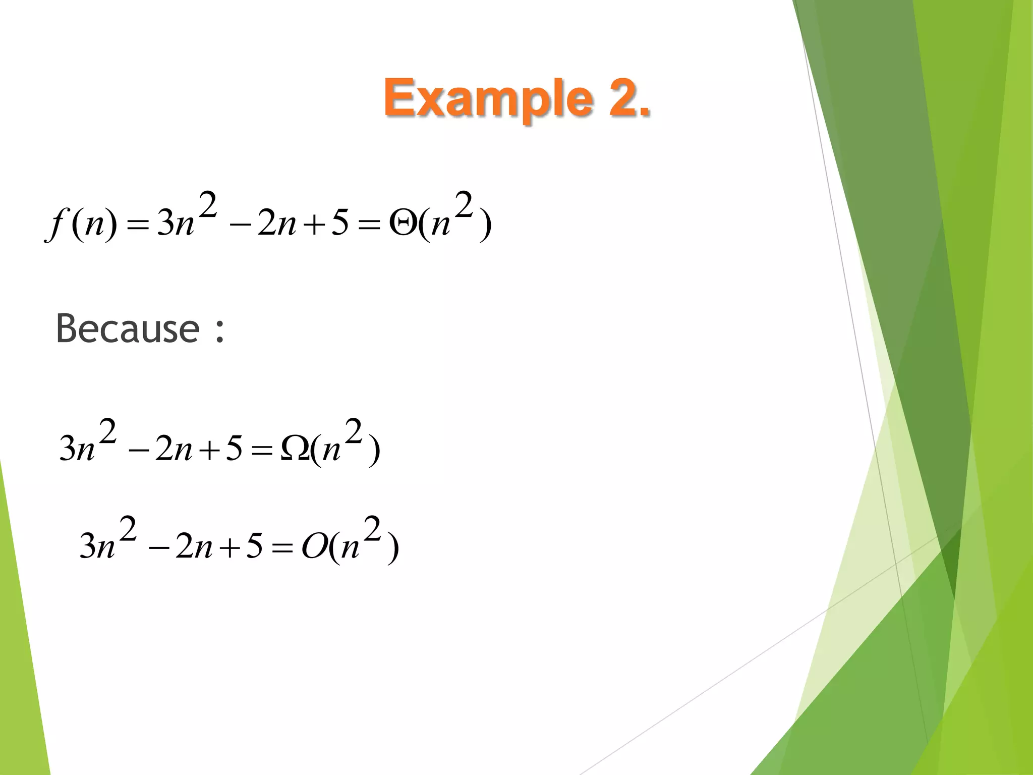
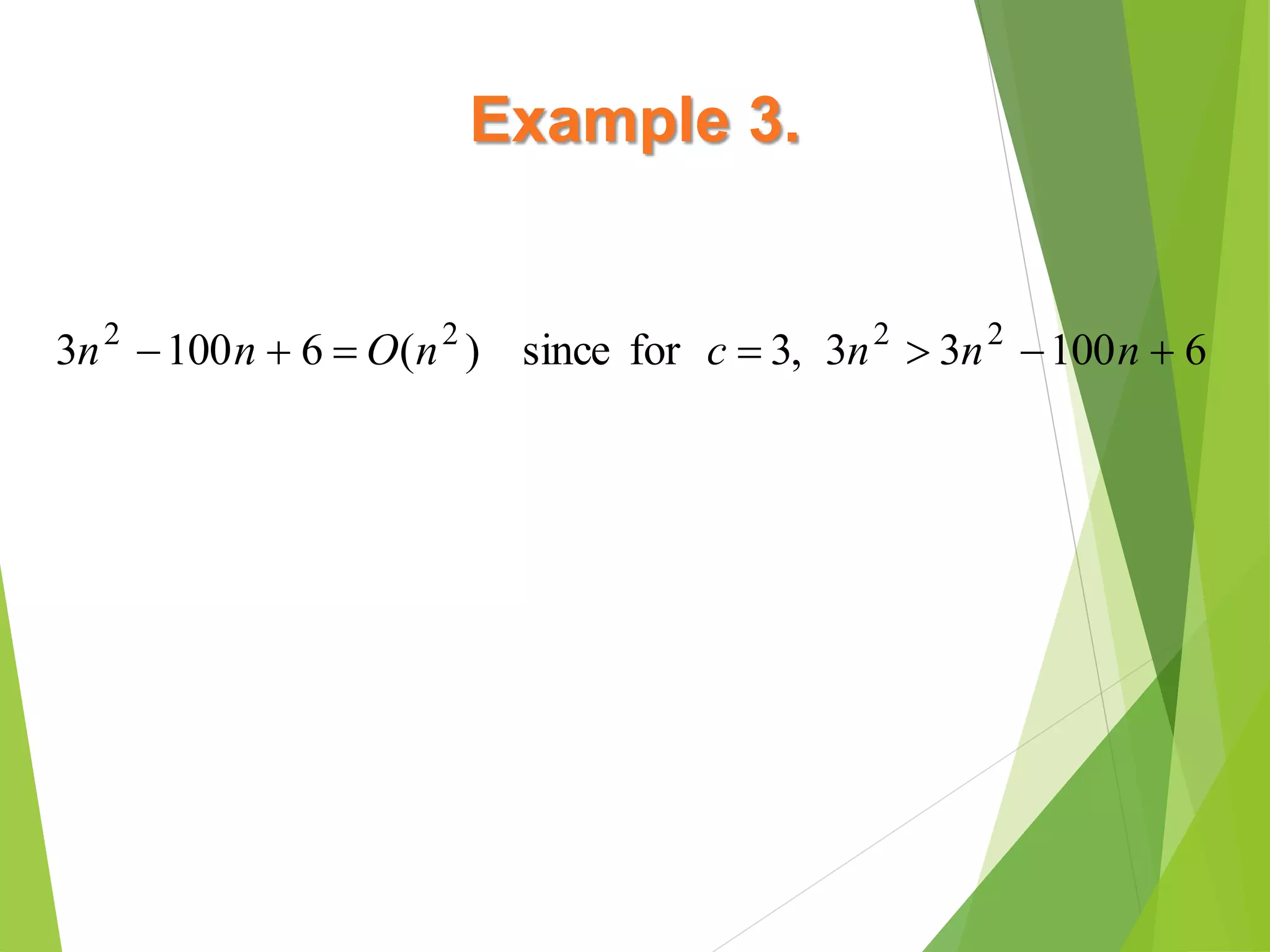
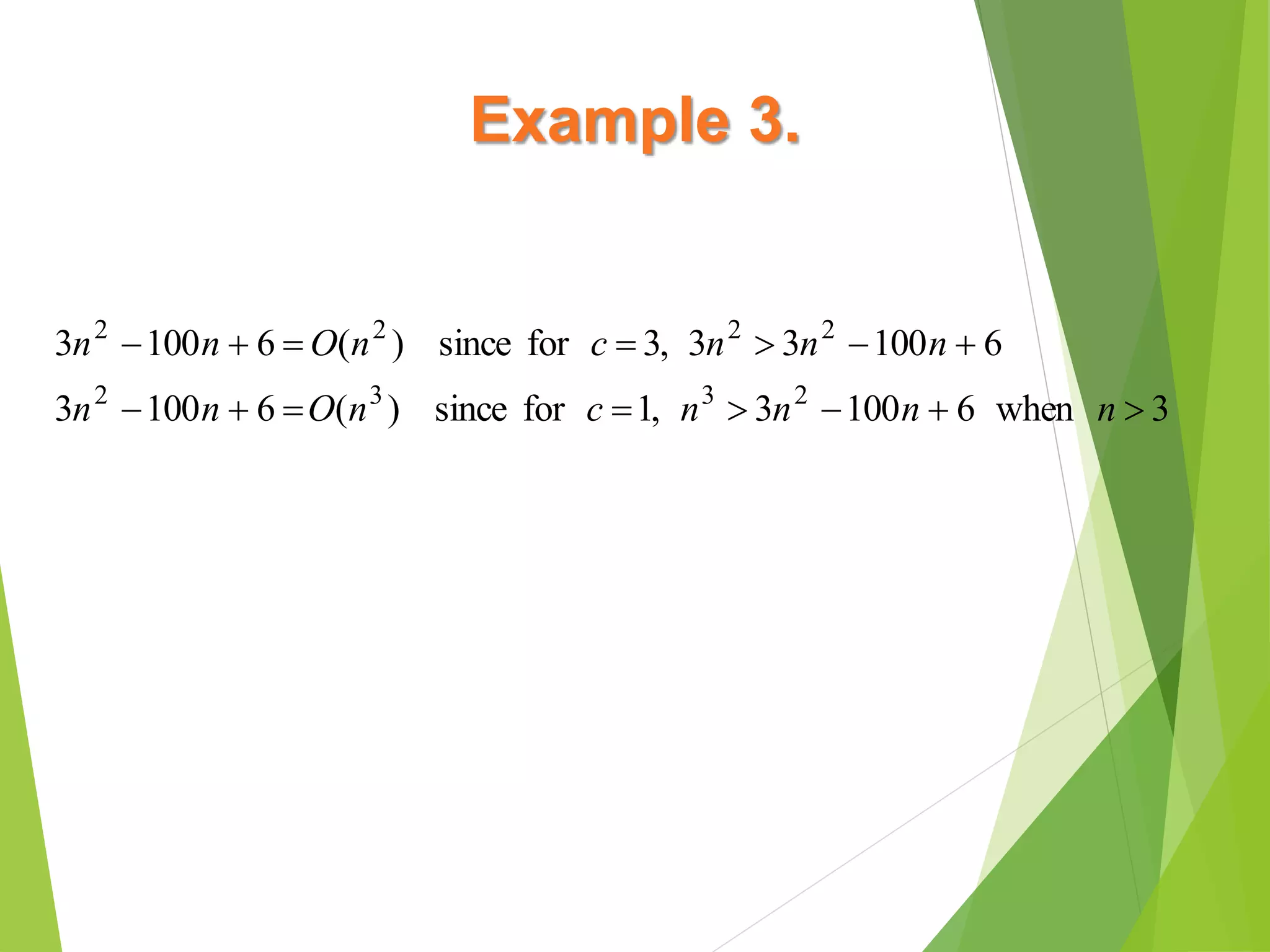
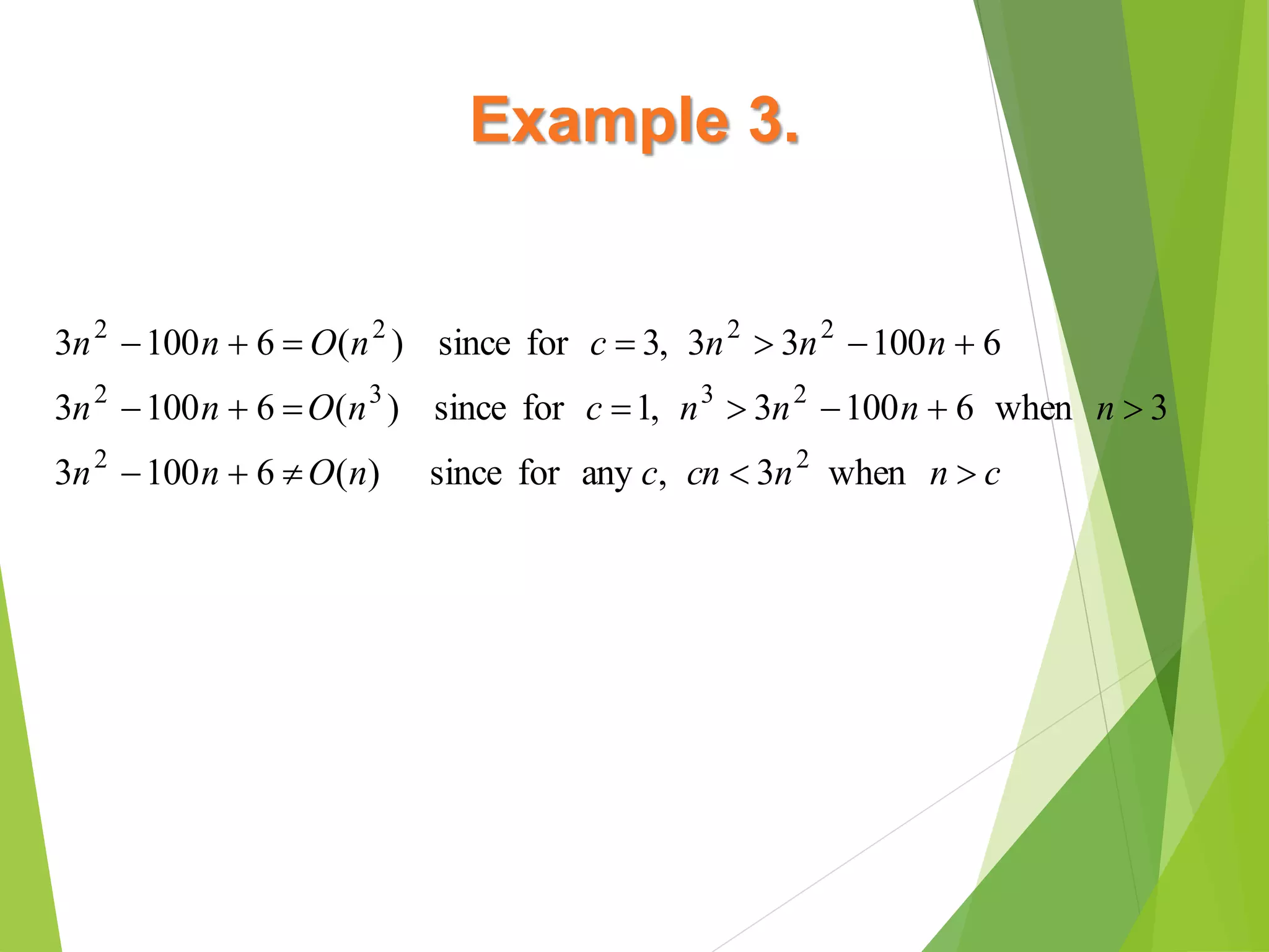
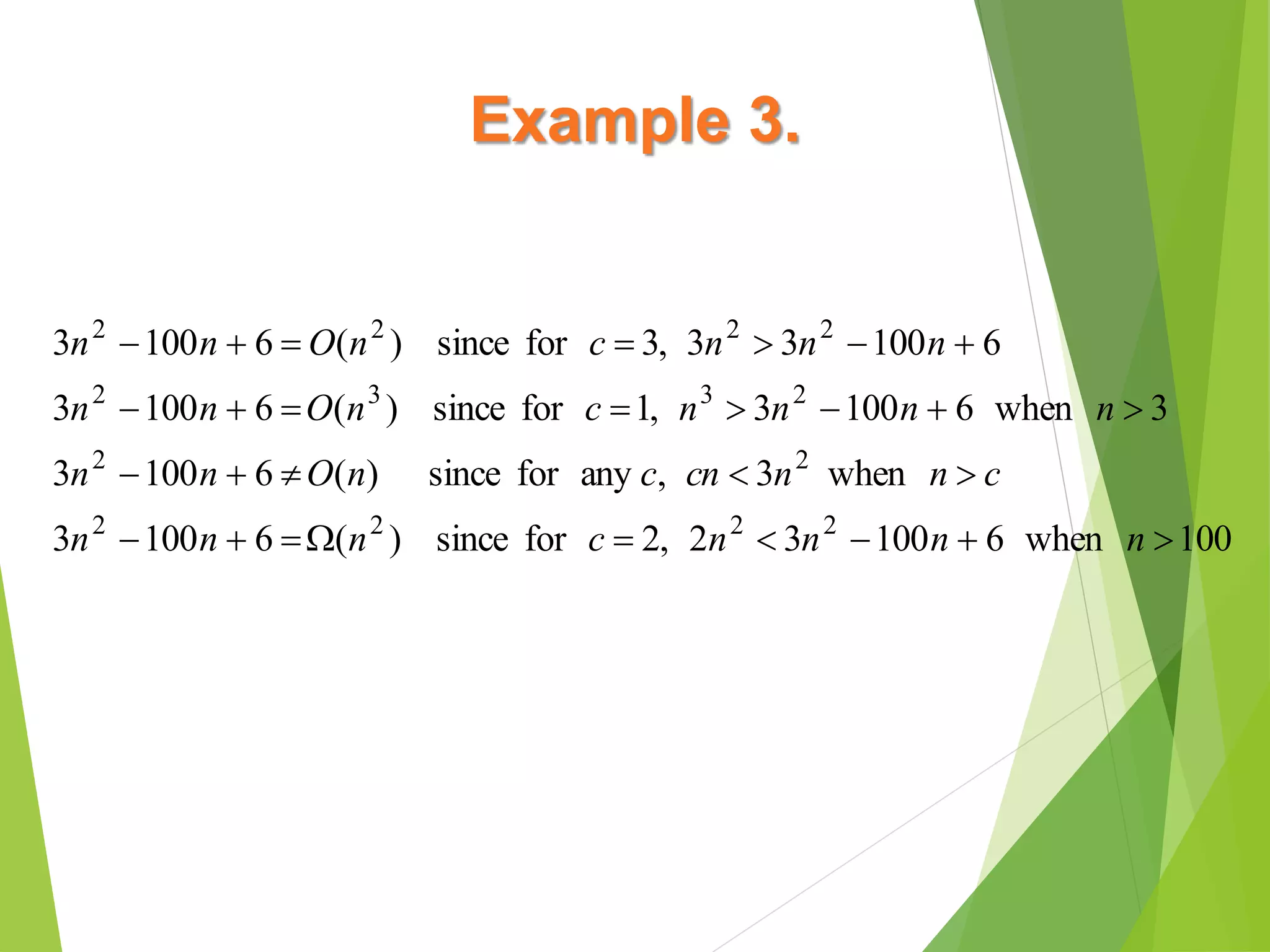
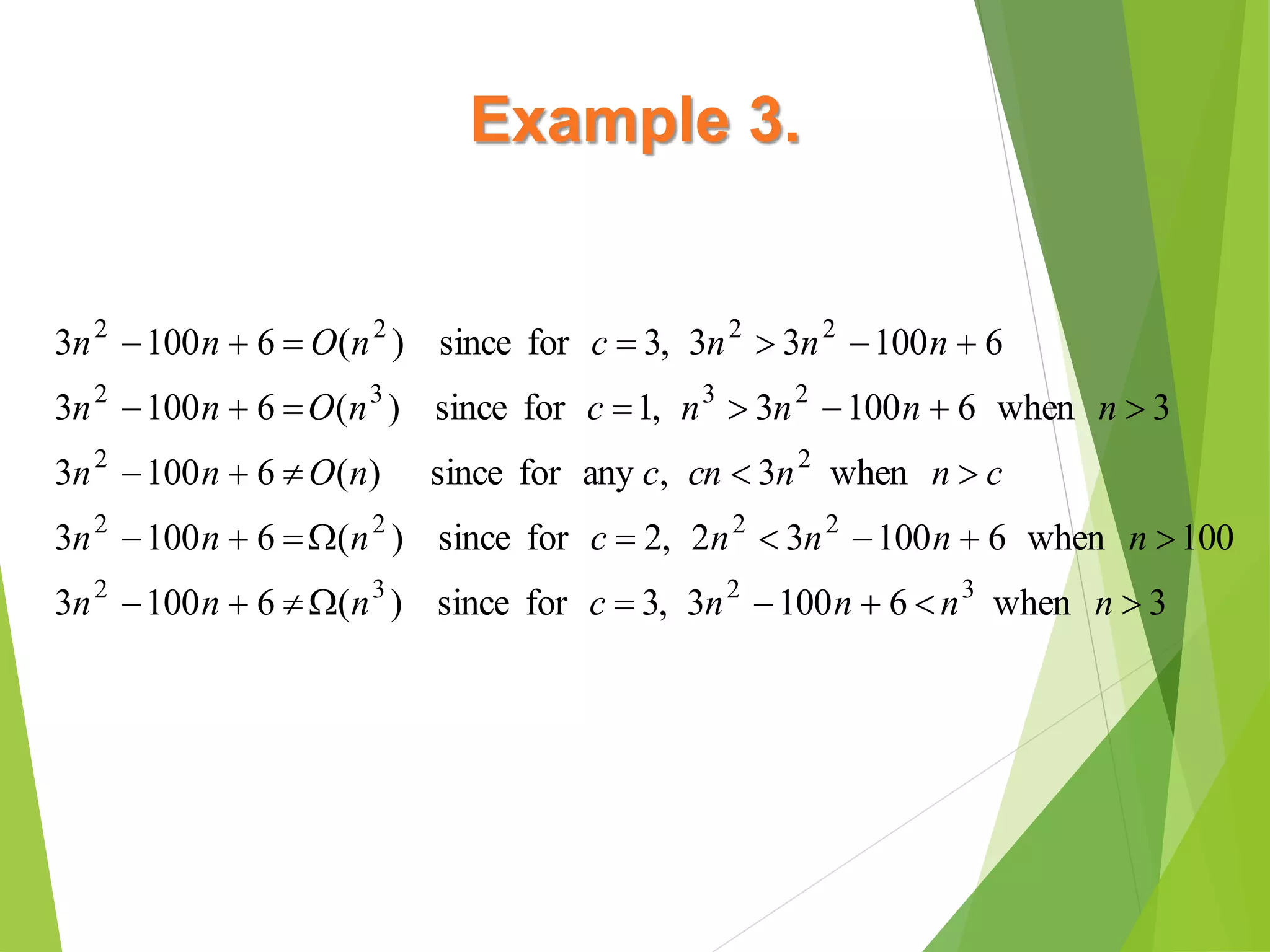
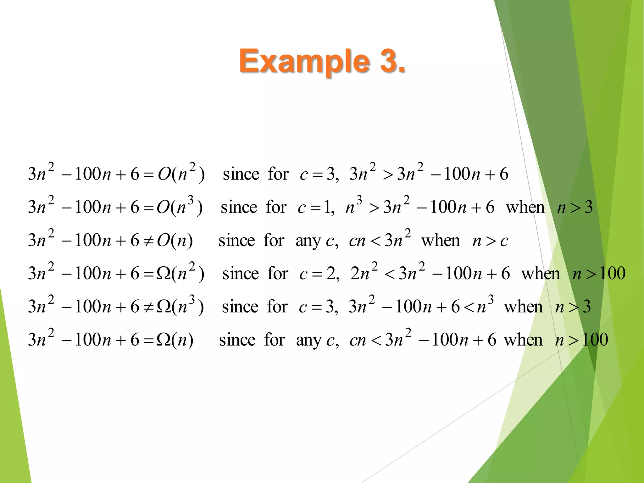
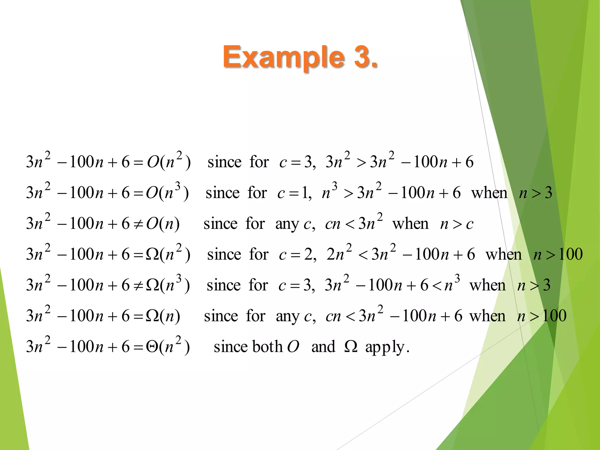
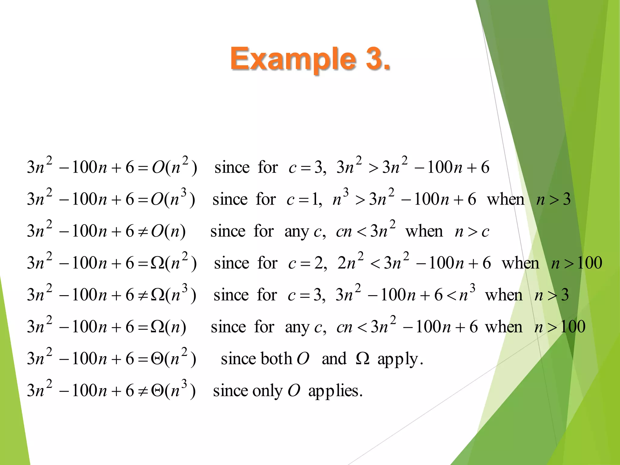


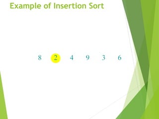
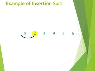
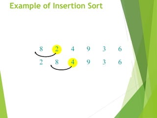
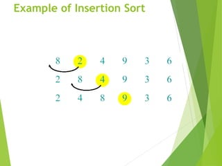
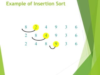
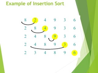
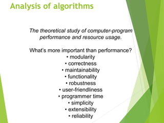
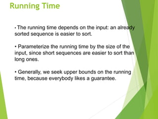
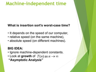
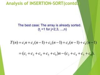
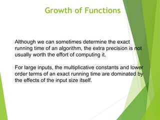
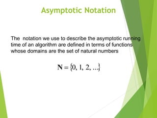
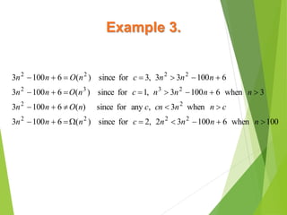
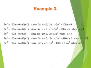
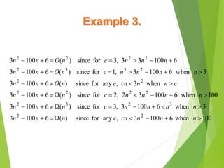
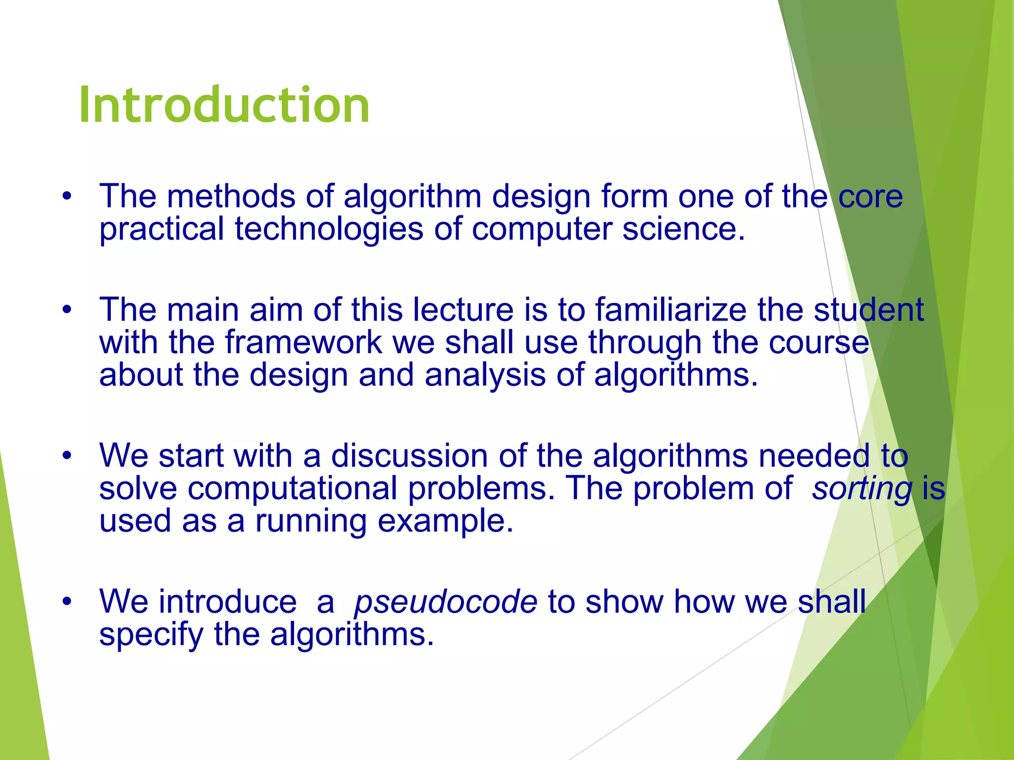
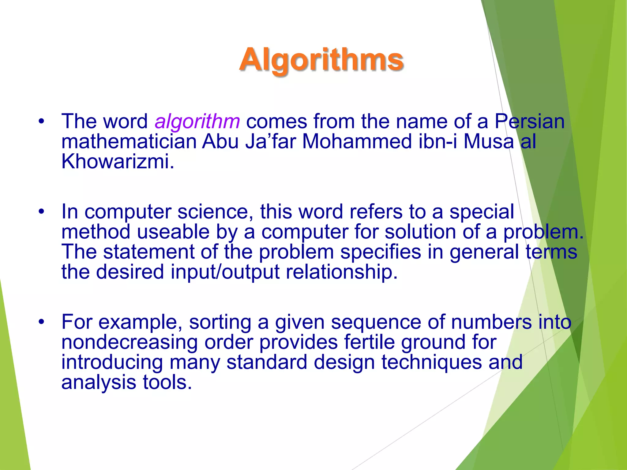
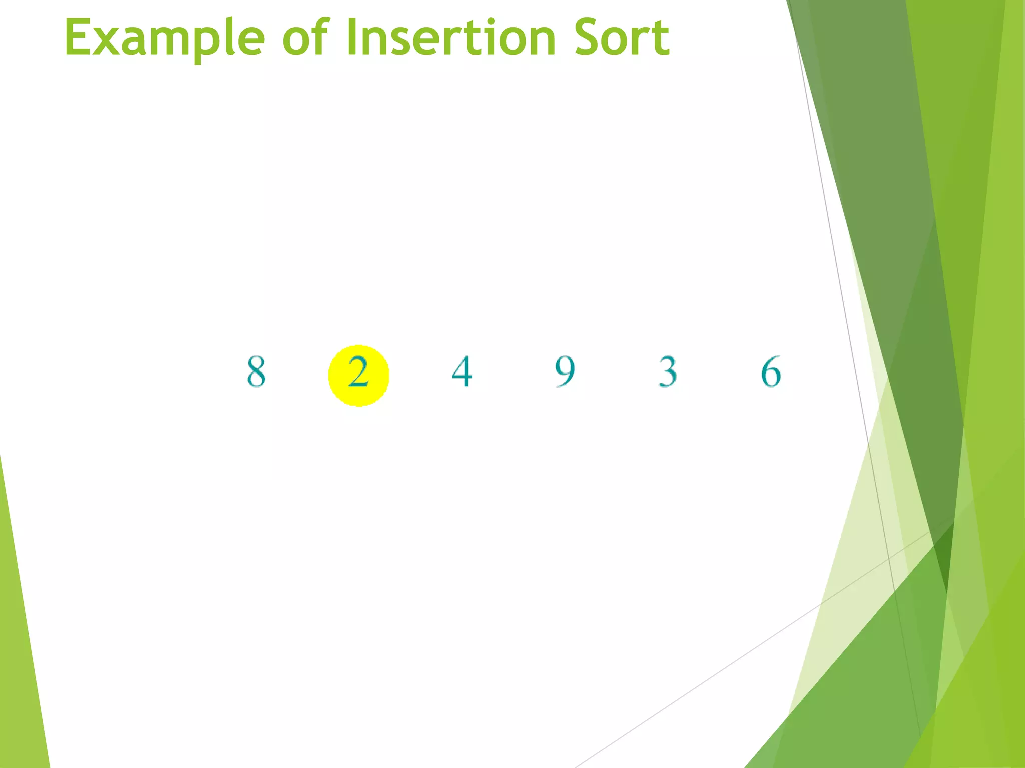
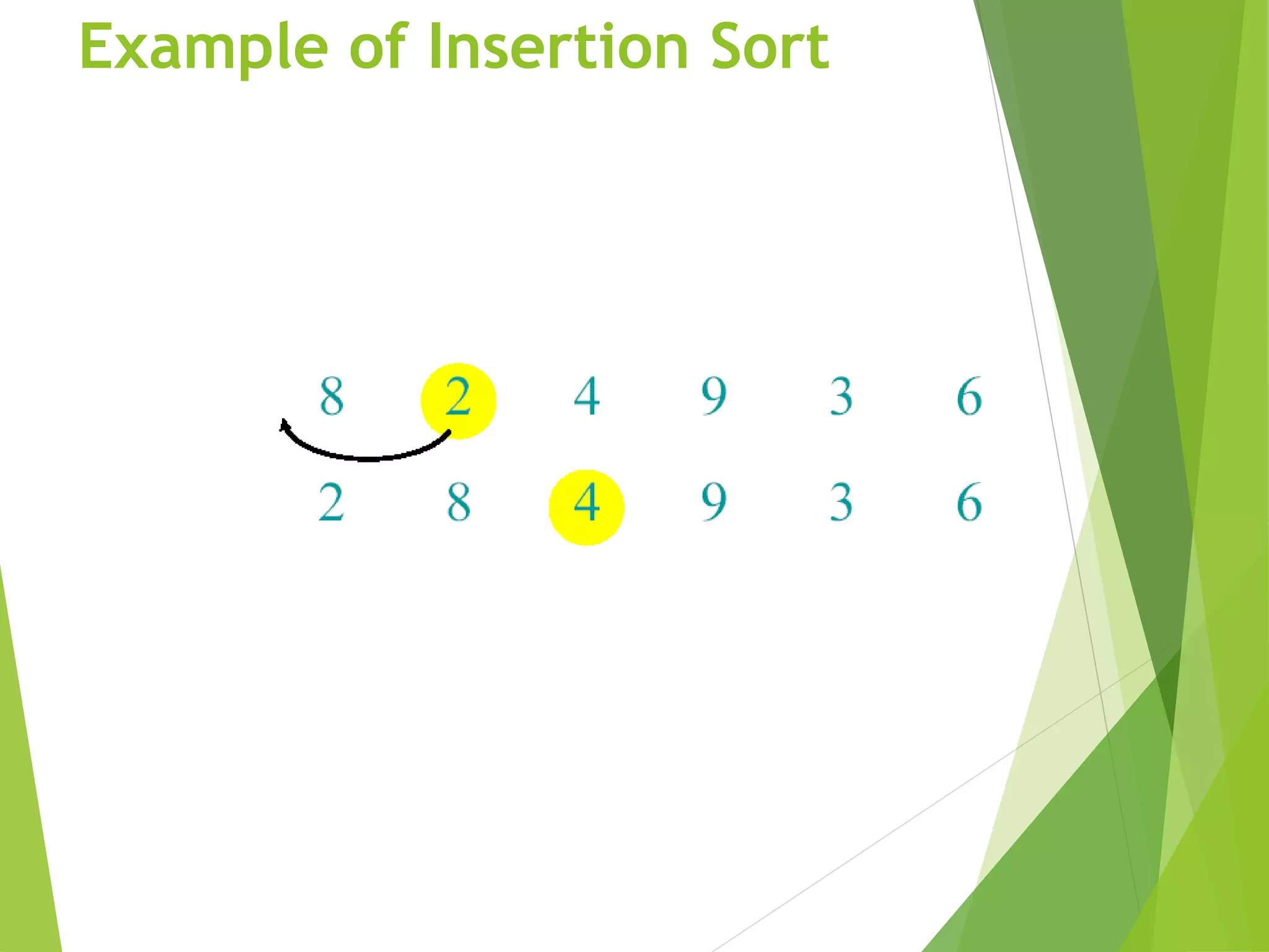
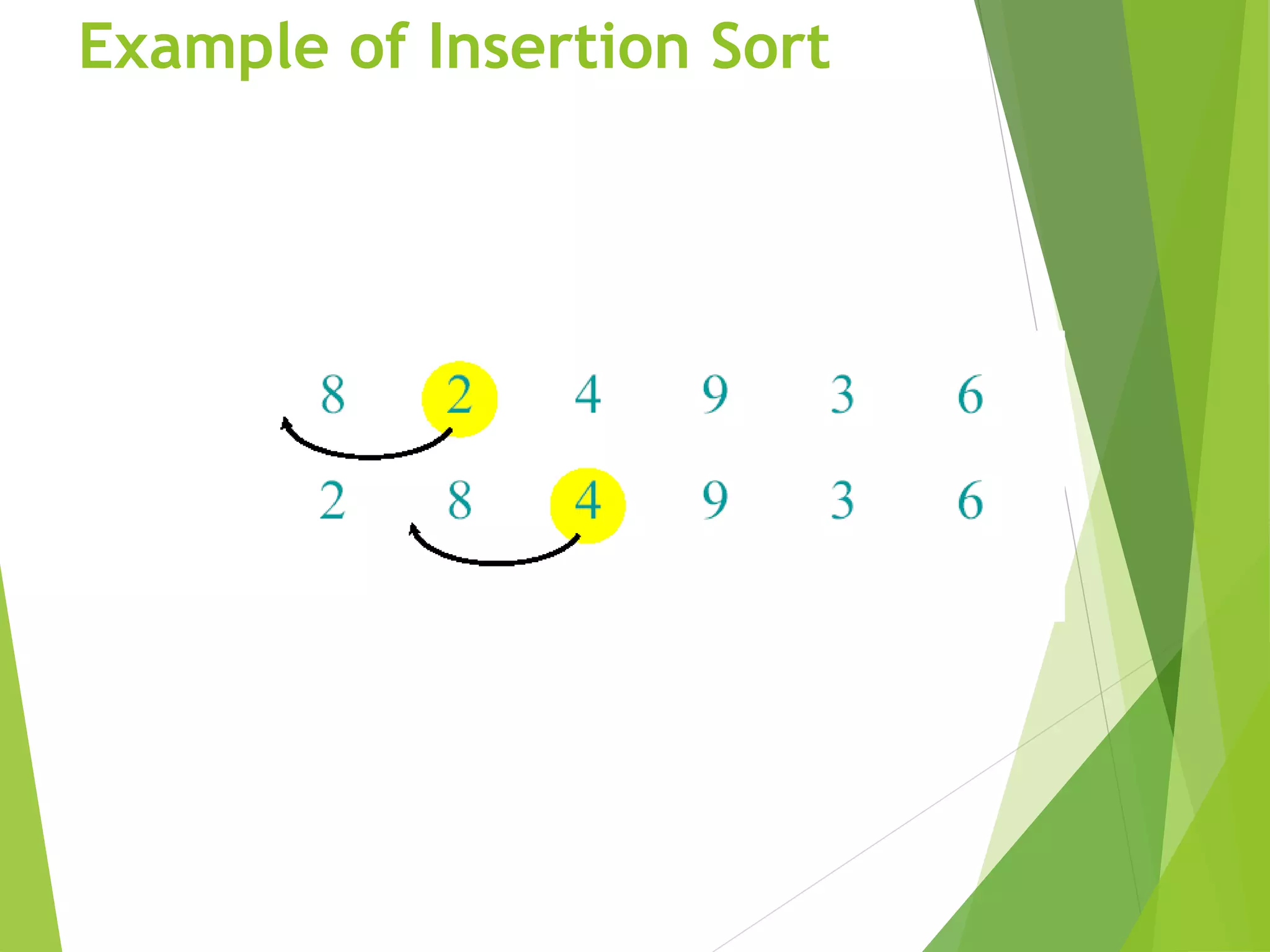
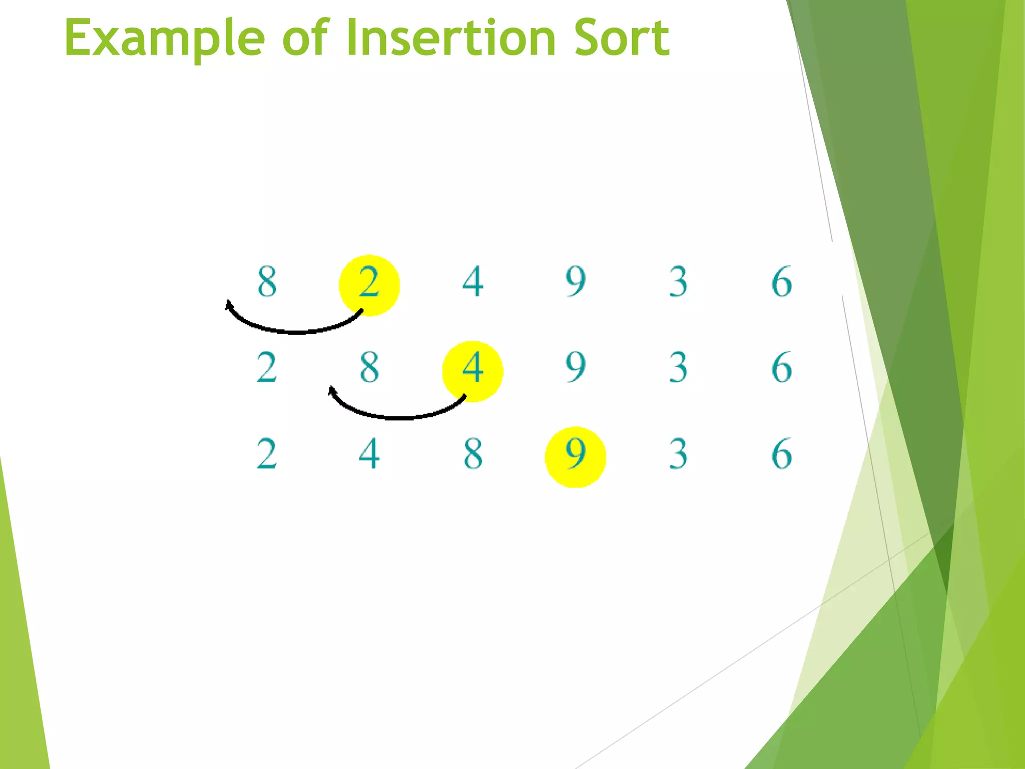
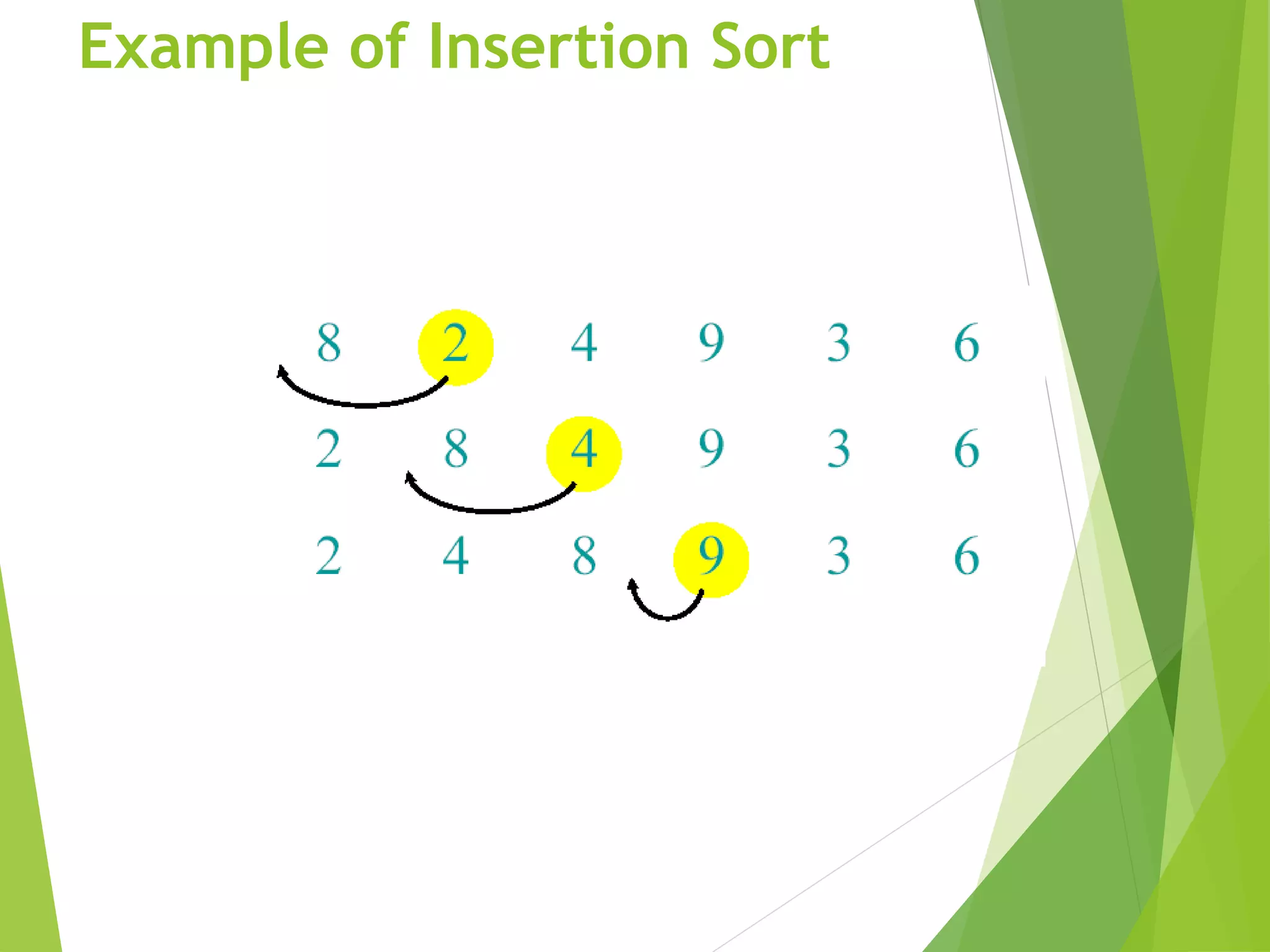
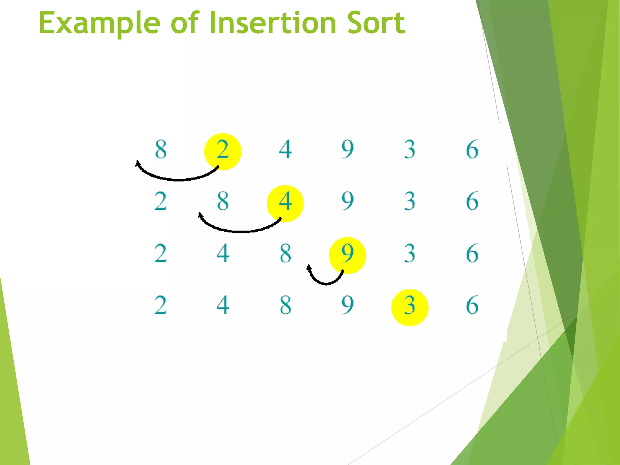
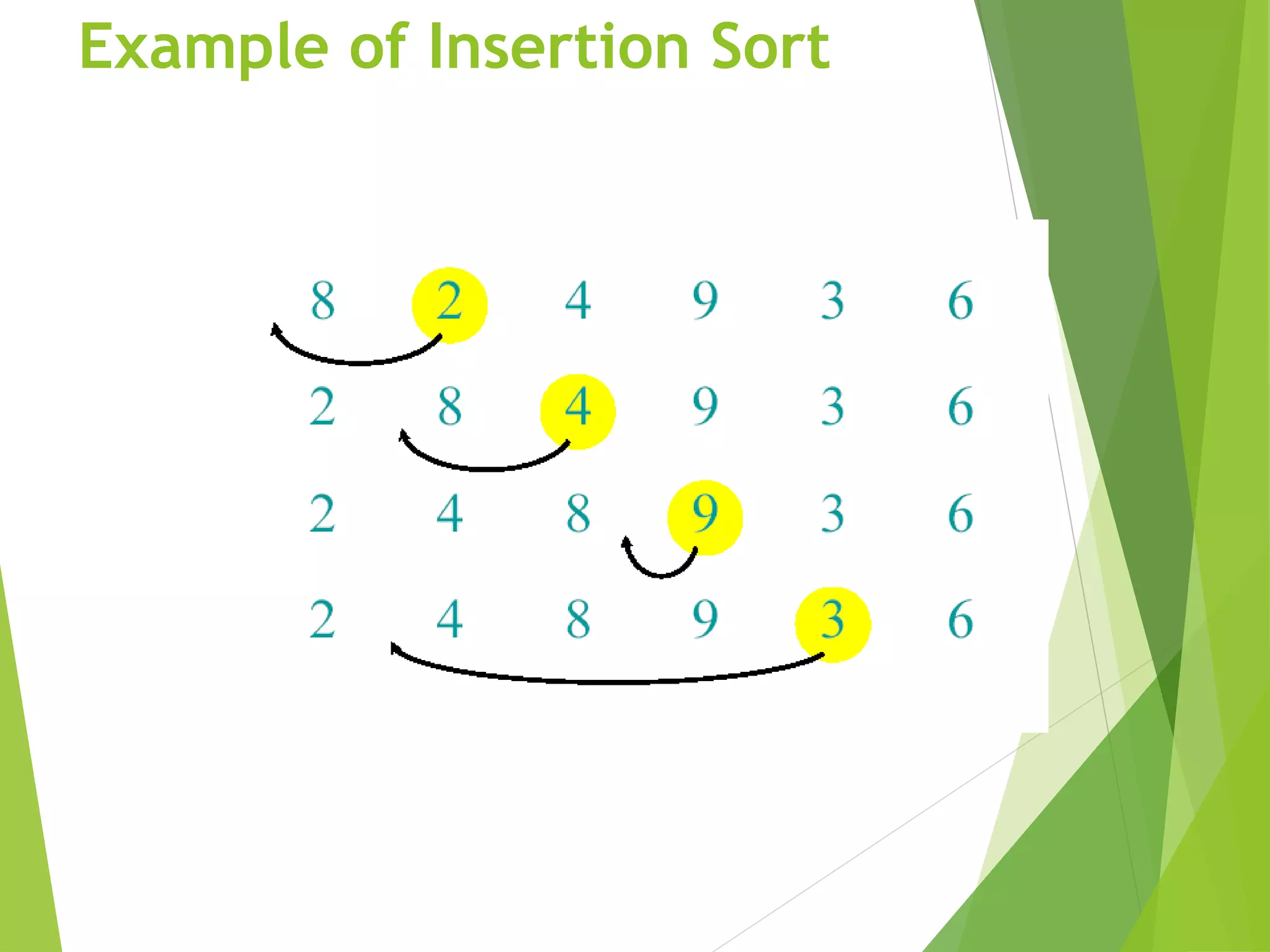
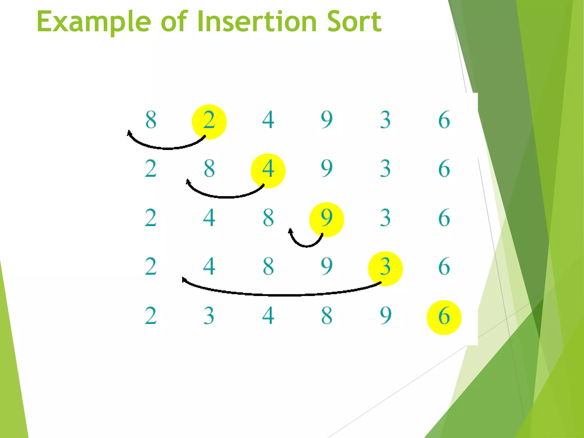
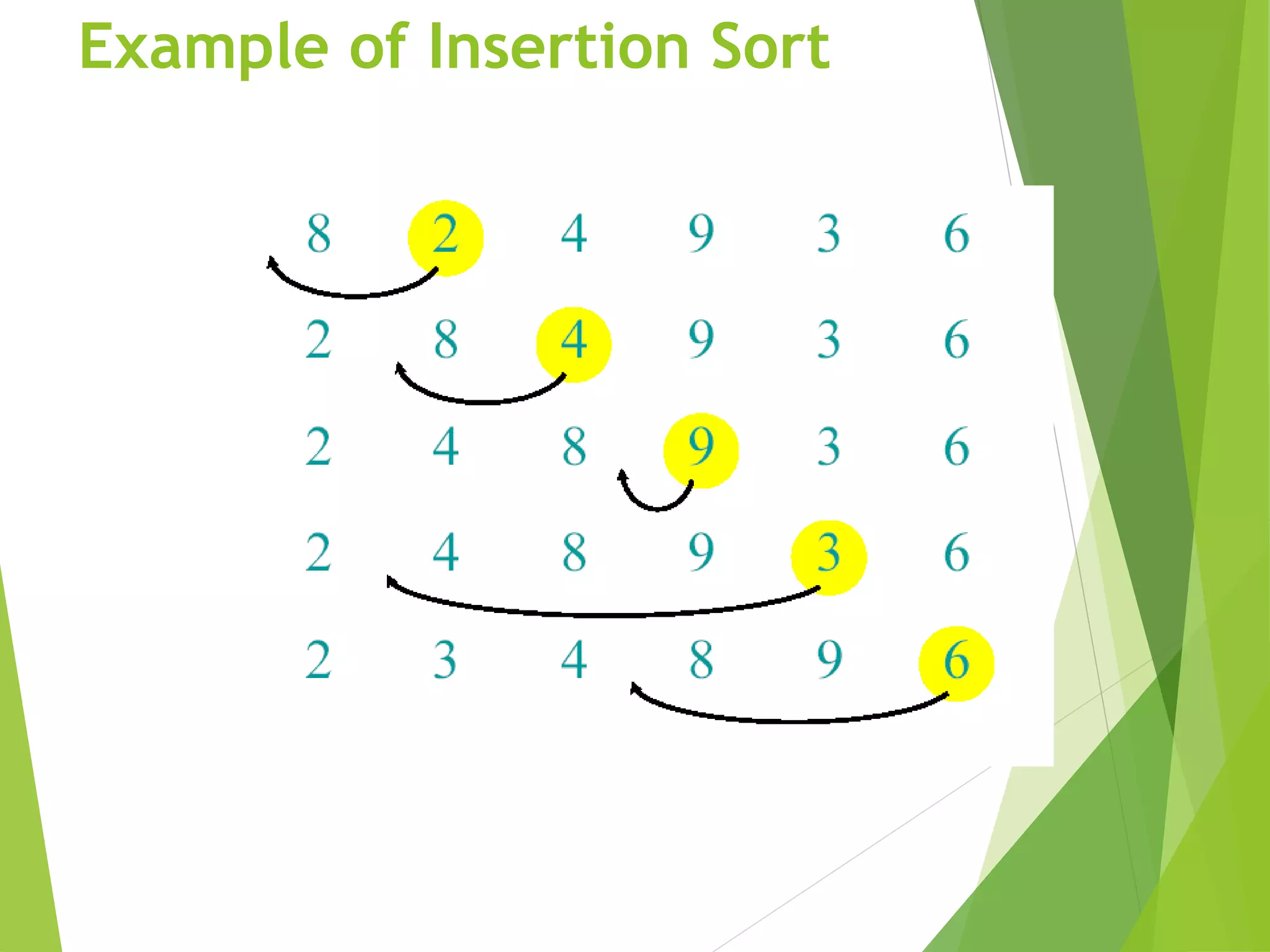
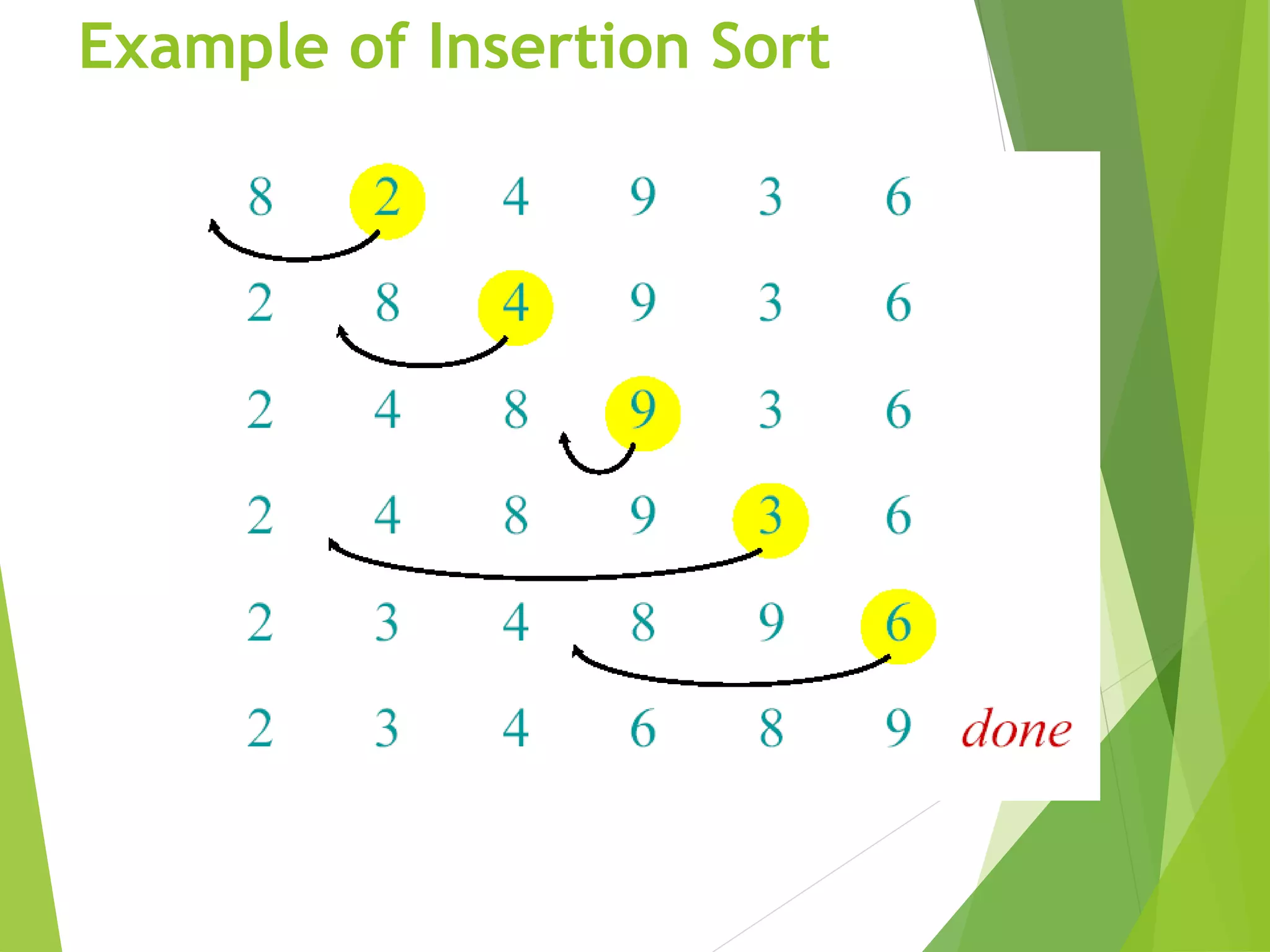
The document discusses algorithms and their analysis. It begins by introducing algorithms and their importance in computer science. The problem of sorting is used as an example to introduce algorithms. Insertion sort is presented as a basic sorting algorithm, with examples of how it works. The analysis of algorithms is then discussed, including analyzing insertion sort's worst case running time, which grows quadratically as Θ(n^2). Asymptotic notation such as O, Ω, Θ is also introduced to analyze long term algorithm running times independent of machine details.


![UiPath Automation Suite Installation (Hands-On) [2/3]](https://cdn.slidesharecdn.com/ss_thumbnails/automationsuitecommunitysession2-251015095633-a6d862f1-thumbnail.jpg?width=600ounds&width=560&fit=bounds)


