
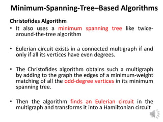
Downloaded 17 times

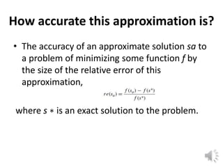


![Multifragment-heuristic algorithm
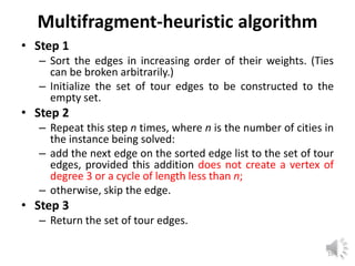
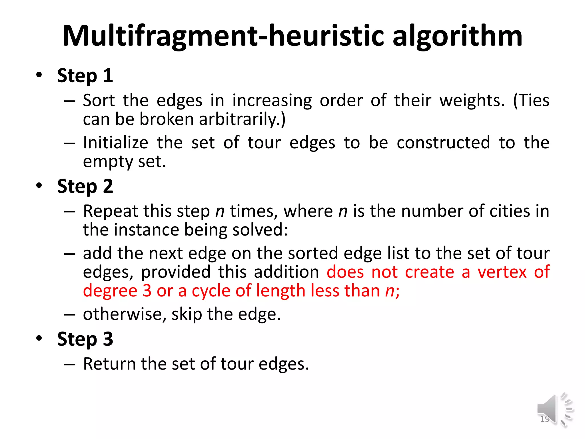
• This method is applied to Eucledian Graphs
which follows the below conditions:
– triangle inequality d[i, j ]≤ d[i, k]+ d[k, j] for any
triple of cities i, j, and K
– symmetry d[i, j ]= d[j, i] for any pair of cities i and j
• Accuracy ratio satisfy the following inequality
21](https://image.slidesharecdn.com/approximationalgorithms-tsp-200417065322/85/Approximation-Algorithms-TSP-21-320.jpg)


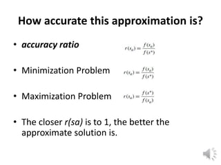
![Multifragment-heuristic algorithm
• This method is applied to Eucledian Graphs
which follows the below conditions:
– triangle inequality d[i, j ]≤ d[i, k]+ d[k, j] for any
triple of cities i, j, and K
– symmetry d[i, j ]= d[j, i] for any pair of cities i and j
• Accuracy ratio satisfy the following inequality
21](https://image.slidesharecdn.com/approximationalgorithms-tsp-200417065322/75/Approximation-Algorithms-TSP-21-2048.jpg)


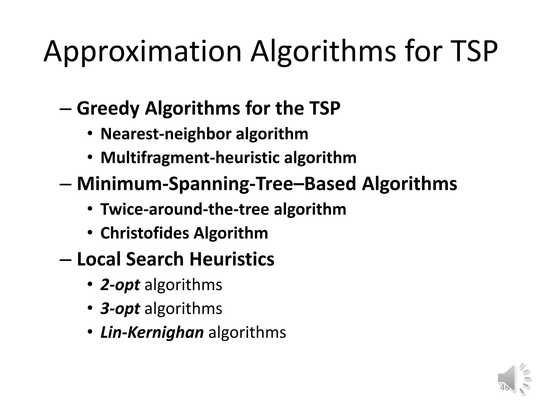
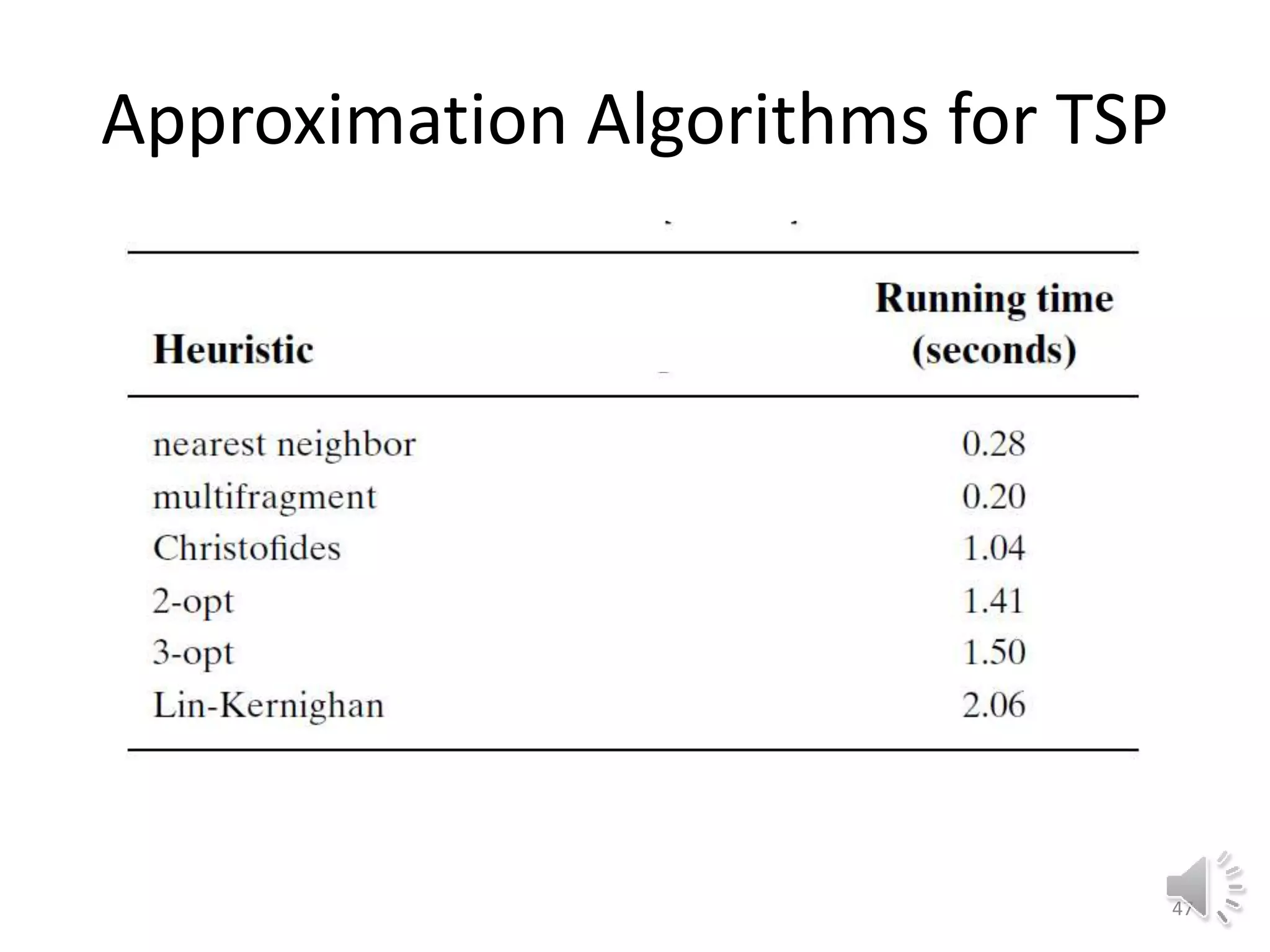

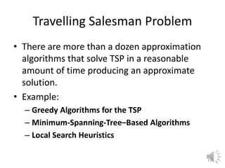
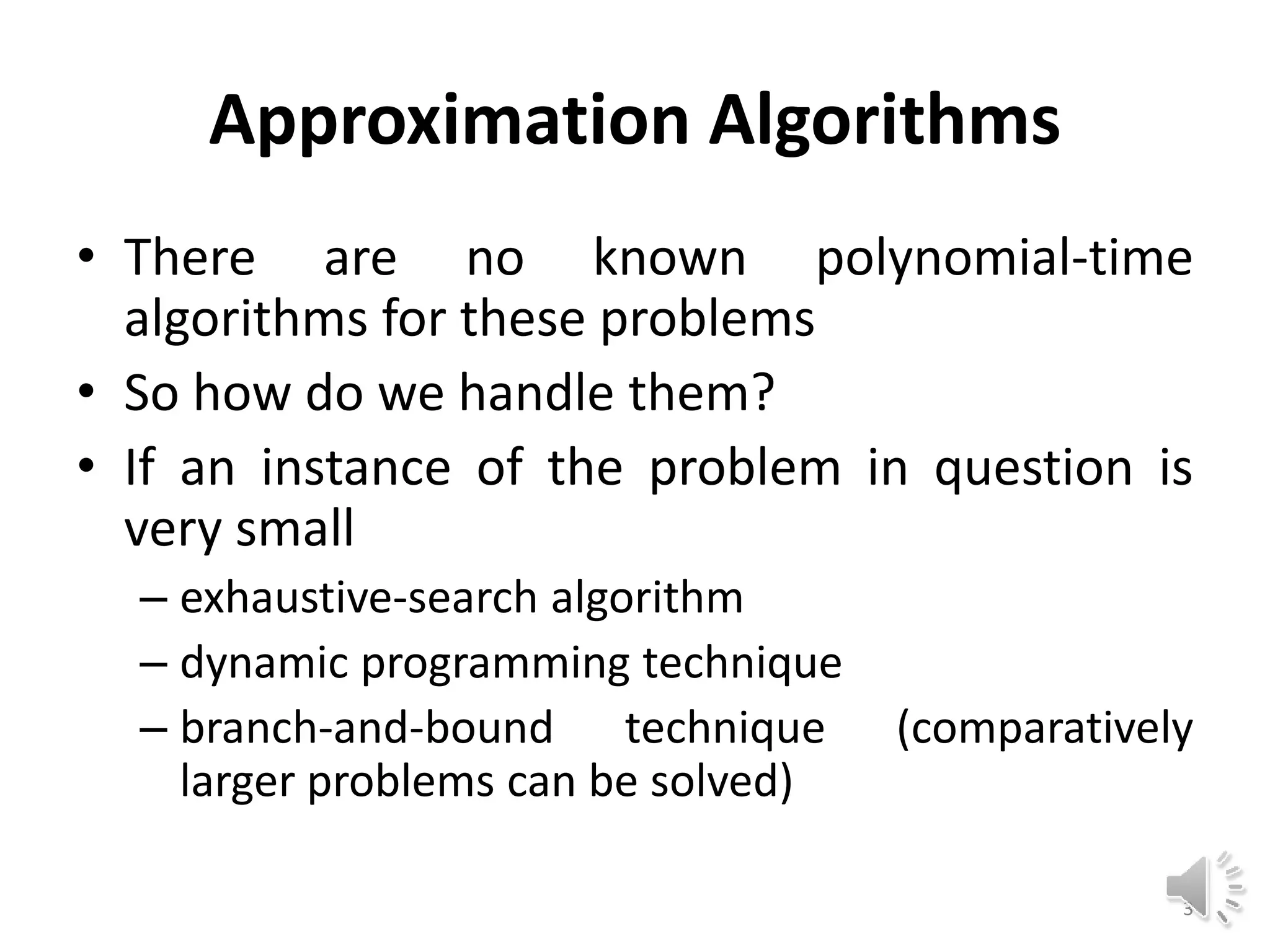
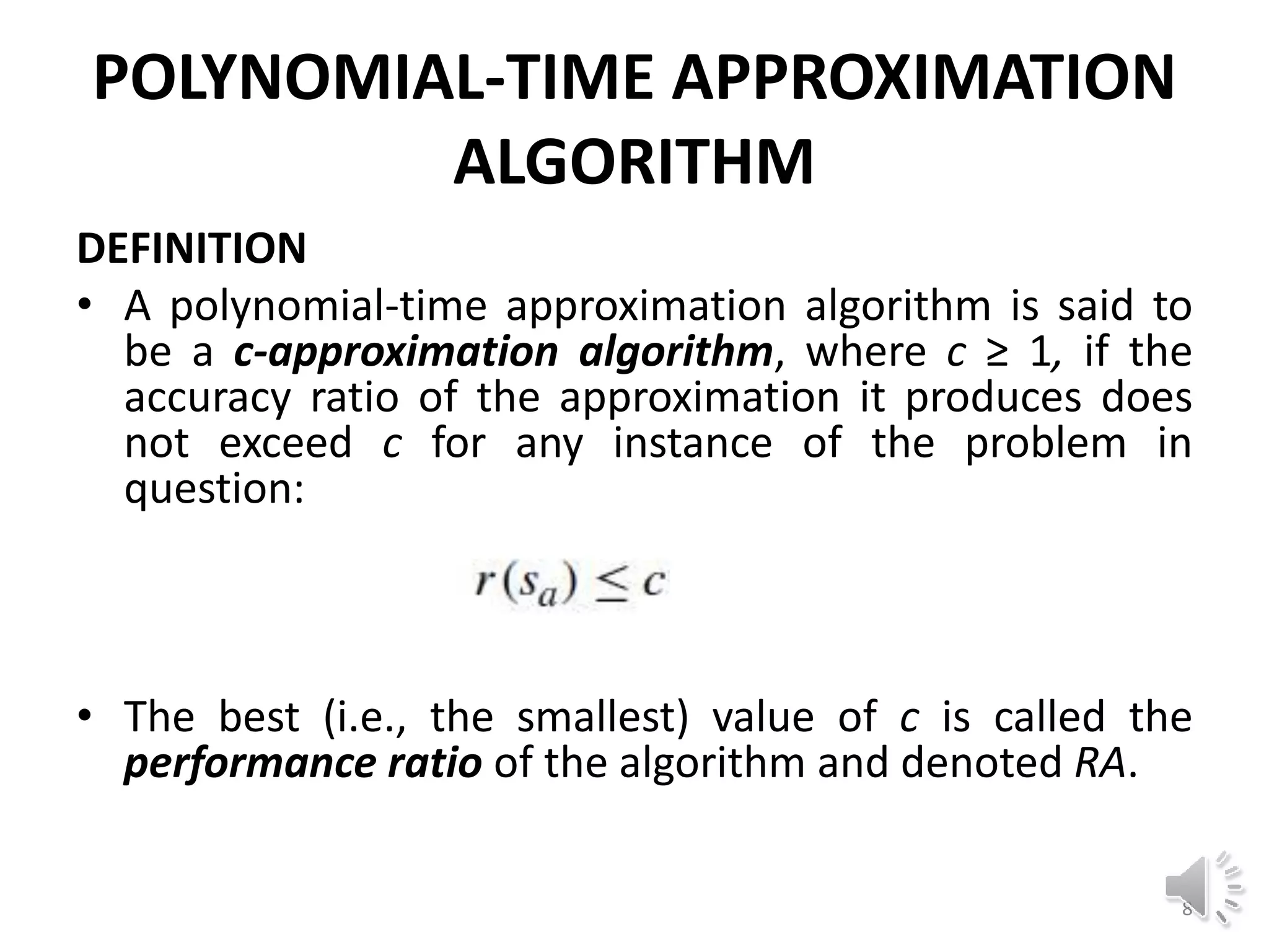
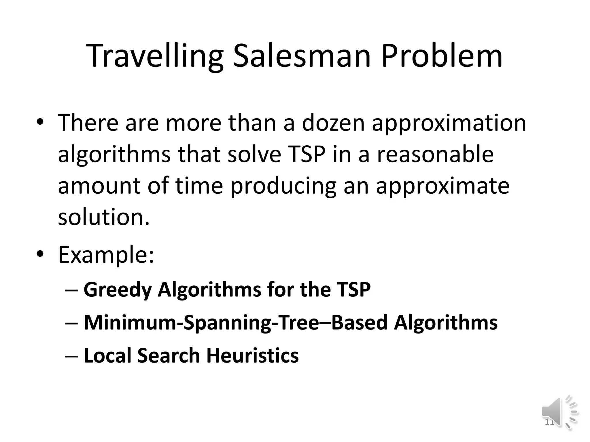
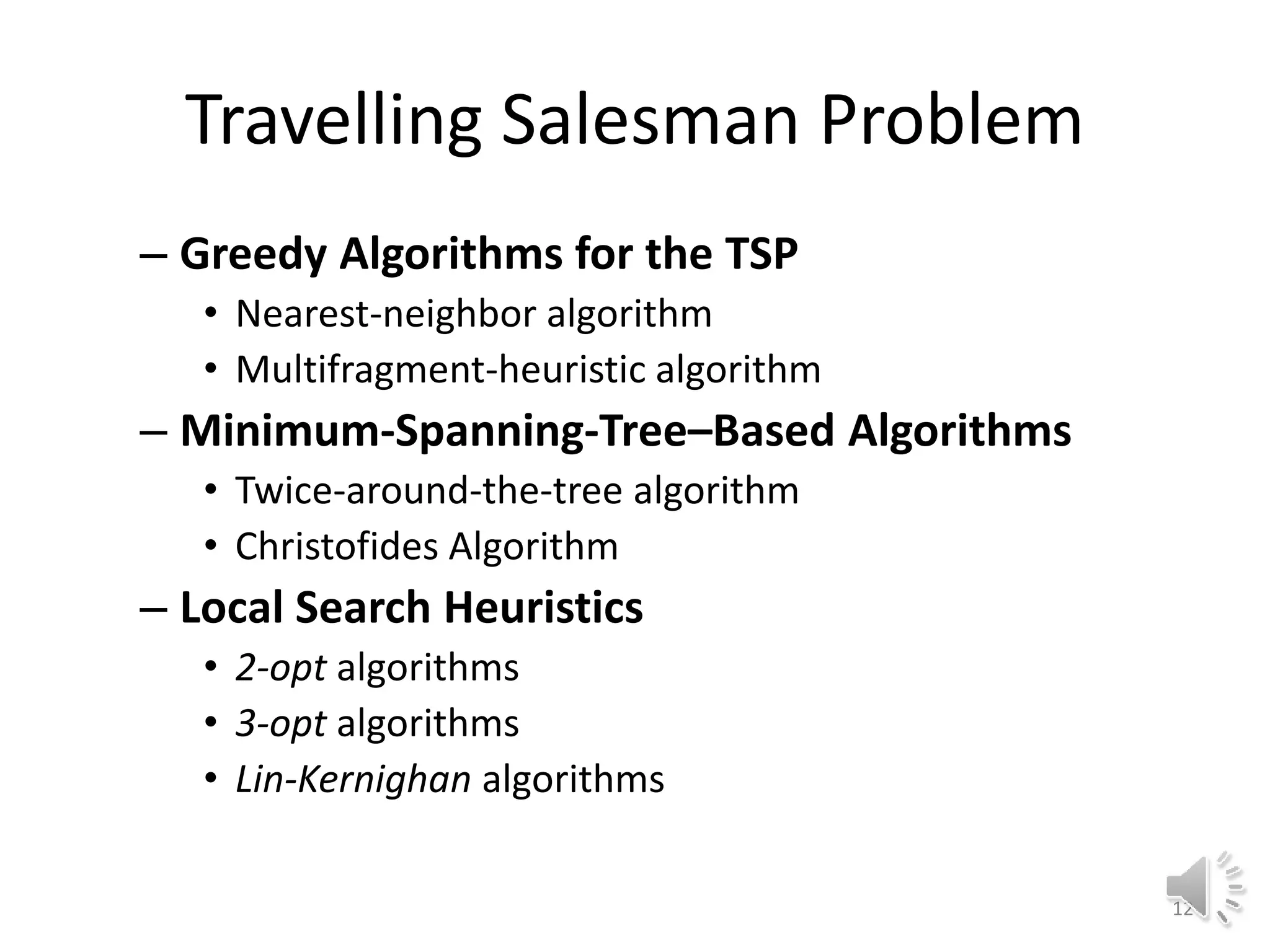
This document discusses approximation algorithms for solving NP-hard problems like the traveling salesman problem (TSP) and knapsack problem. It provides an overview of approximation algorithms, defining them as polynomial-time algorithms that provide good but not necessarily optimal solutions. The document then focuses on approximation algorithms for the TSP, describing greedy algorithms like nearest neighbor, minimum spanning tree based algorithms like Christofides, and local search heuristics like 2-opt and Lin-Kernighan. It concludes by noting some applications of approximating the TSP.


