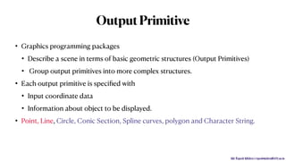
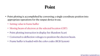
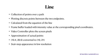
Download as PDF, PPTX


![Mr. Rupesh Mishra | rupeshmishra@sfit.ac.in
du
dl
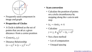
Decisión parameter
y = mx + c
y = m(xk + 1) + c
dl = y − yk = [m(xk + 1) + c] − yk
du = yk+1 − y = yk+1 − [m(xk + 1) + c]
if(dl − du < 0) − > yk
if(dl − du > 0) − > yk+1
xk
yk+1
yk
xk+1
y](https://image.slidesharecdn.com/2-201016145559/85/Computer-Graphics-Output-Primitive-18-320.jpg)
![Mr. Rupesh Mishra | rupeshmishra@sfit.ac.in
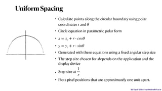
dl − du = [[m(xk + 1) + c] − yk] − [yk+1 − [m(xk + 1) + c]]
dl − du = m(xk + 1) + c − yk − yk+1 + m(xk + 1) − c
dl − du = 2m(xk + 1) − 2yk + 2c − 1
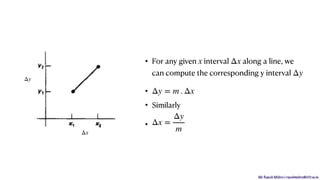
m =
Δy
Δx
dl − du =
2Δy
Δx
(xk + 1) − 2yk + 2c − 1
dl − du = Δx[
2Δy
Δx
(xk + 1) − 2yk + 2c − 1]
Δx(dl − du) = 2Δy(xk + 1) − 2Δxyk + 2Δxc − Δx
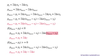
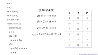
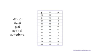
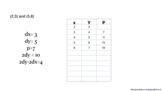
pk = Δx(dl − du) = 2Δyxk + 2Δy − 2Δxyk + 2Δxc − Δx
pk = Δx(dl − du) = 2Δyxk − 2Δxyk](https://image.slidesharecdn.com/2-201016145559/85/Computer-Graphics-Output-Primitive-19-320.jpg)
![Mr. Rupesh Mishra | rupeshmishra@sfit.ac.in
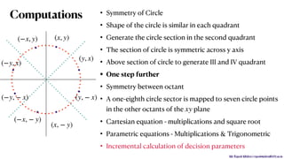
InitialDecisionParameter
p0 = 2Δyx1 + 2Δy − 2Δxy1 + 2Δxc − Δx
c = y −
Δy
Δx
x1
p0 = 2Δyx1 + 2Δy − 2Δxy1 + 2Δx[y −
Δy
Δx
x1] − Δx
p0 = 2Δyx1 + 2Δy − 2Δxy1 + 2Δxy1 − 2Δyx1 − Δx
p0 = 2Δy − Δx](https://image.slidesharecdn.com/2-201016145559/85/Computer-Graphics-Output-Primitive-21-320.jpg)


![Mr. Rupesh Mishra | rupeshmishra@sfit.ac.in
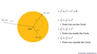
Midpoint
midpoint = [
xk+1 + xk+1
2
,
yk + yk−1
2
]
midpoint = [
xk + 1 + xk + 1
2
,
yk + yk − 1
2
]
midpoint = [xk + 1,yk −
1
2
]
midpoint = [xk+1, yk− 1
2
]
midpoint = [xm, ym]
(xk + 1,yk)
(xk + 1,yk − 1)
.
.](https://image.slidesharecdn.com/2-201016145559/85/Computer-Graphics-Output-Primitive-35-320.jpg)
![Mr. Rupesh Mishra | rupeshmishra@sfit.ac.in
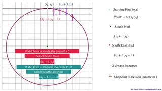
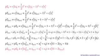
Decision Parameter
midpoint = [xm, ym]
(pk)
pk = x2
m + y2
m − r2
pk = x2
k+1 + y2
k− 1
2
− r2
pk+1 = (xk+1 + 1)2
+ (yk+1 −
1
2
)2
− r2
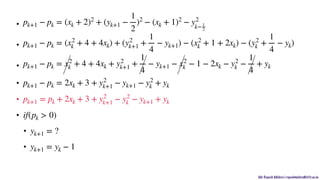
pk+1 − pk = (xk+1 + 1)2
+ (yk+1 −
1
2
)2
− r2
− x2
k+1 − y2
k−1
2
+ r2
pk+1 − pk = (xk + 1 + 1)2
+ (yk+1 −
1
2
)2
− (xk + 1)2
− y2
k−1
2
pk+1 − pk = (xk + 2)2
+ (yk+1 −
1
2
)2
− (xk + 1)2
− y2
k−1
2](https://image.slidesharecdn.com/2-201016145559/85/Computer-Graphics-Output-Primitive-36-320.jpg)


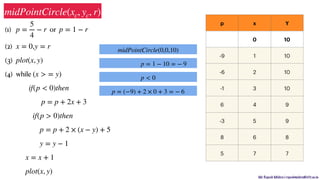


![Mr. Rupesh Mishra | rupeshmishra@sfit.ac.in
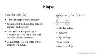
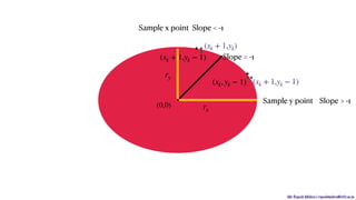
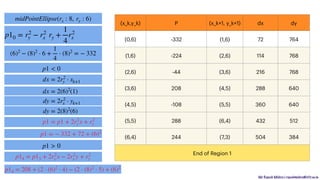
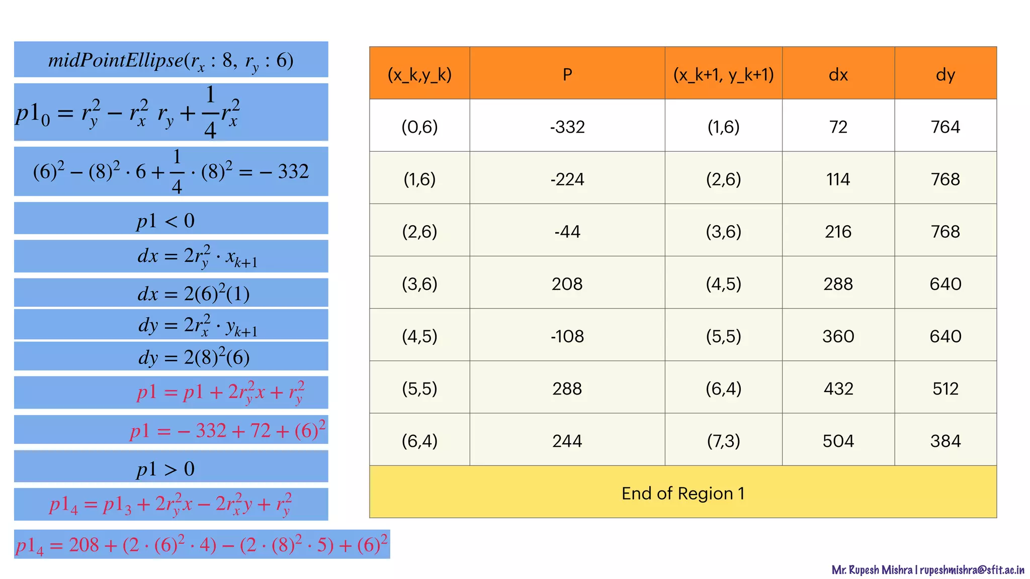
[Region I]
• Previous position
• Sampling position
• Midpoint between the two
candidate pixels
•
• Evaluating the decision parameterat
midpoint
•
•
•
• Mid point is inside the ellipse
•
•
• Mid point is on the ellipse
•
•
• Mid point is outside the ellipse
•
(xk, yk)
xk+1
(xk + 1,yk) (xk + 1,yk − 1)
Mid Point (xk + 1,yk −
1
2
)
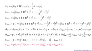
p1k = r2
y (xk + 1)2
+ r2
x (yk −
1
2
)2
− r2
x r2
y
if (p1k < 0)
(xk + 1,yk)
if (p1k = 0)
(xk + 1,yk − 1)
if (p1k > 0)
(xk + 1,yk − 1)](https://image.slidesharecdn.com/2-201016145559/85/Computer-Graphics-Output-Primitive-54-320.jpg)
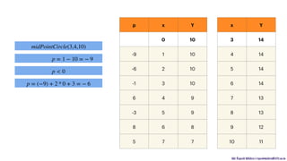
![Mr. Rupesh Mishra | rupeshmishra@sfit.ac.in
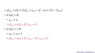
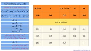
[Region II]
• Previous position
• Sampling position
• Midpoint between the two
candidate pixels
•
• Evaluating the decision parameter
at midpoint
•
•
•
• Mid point is inside the ellipse
•
•
• Mid point is on the ellipse
•
•
• Mid point is outside the ellipse
•
(xk, yk)
yk+1
(xk, yk − 1) (xk + 1,yk − 1)
Mid Point (xk +
1
2
, yk − 1)
p2k = r2
y (xk +
1
2
)2
+ r2
x (yk − 1)2
− r2
x r2
y
if (p2k < 0)
(xk + 1,yk − 1)
if (p2k = 0)
(xk, yk − 1)
if (p2k > 0)
(xk, yk − 1)](https://image.slidesharecdn.com/2-201016145559/85/Computer-Graphics-Output-Primitive-59-320.jpg)
![Mr. Rupesh Mishra | rupeshmishra@sfit.ac.in
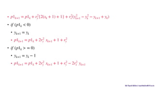
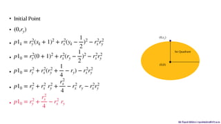
InitialPoint
• Last Point of [Region I]
• Let
•
•
(x, y)
p2k = r2
y (xk +
1
2
)2
+ r2
x (yk − 1)2
− r2
x r2
y
p20 = r2
y (x +
1
2
)2
+ r2
x (y − 1)2
− r2
x r2
y](https://image.slidesharecdn.com/2-201016145559/85/Computer-Graphics-Output-Primitive-62-320.jpg)


![Mr. Rupesh Mishra | rupeshmishra@sfit.ac.in
du
dl
Decisión parameter
y = mx + c
y = m(xk + 1) + c
dl = y − yk = [m(xk + 1) + c] − yk
du = yk+1 − y = yk+1 − [m(xk + 1) + c]
if(dl − du < 0) − > yk
if(dl − du > 0) − > yk+1
xk
yk+1
yk
xk+1
y](https://image.slidesharecdn.com/2-201016145559/75/Computer-Graphics-Output-Primitive-18-2048.jpg)
![Mr. Rupesh Mishra | rupeshmishra@sfit.ac.in
dl − du = [[m(xk + 1) + c] − yk] − [yk+1 − [m(xk + 1) + c]]
dl − du = m(xk + 1) + c − yk − yk+1 + m(xk + 1) − c
dl − du = 2m(xk + 1) − 2yk + 2c − 1
m =
Δy
Δx
dl − du =
2Δy
Δx
(xk + 1) − 2yk + 2c − 1
dl − du = Δx[
2Δy
Δx
(xk + 1) − 2yk + 2c − 1]
Δx(dl − du) = 2Δy(xk + 1) − 2Δxyk + 2Δxc − Δx
pk = Δx(dl − du) = 2Δyxk + 2Δy − 2Δxyk + 2Δxc − Δx
pk = Δx(dl − du) = 2Δyxk − 2Δxyk](https://image.slidesharecdn.com/2-201016145559/75/Computer-Graphics-Output-Primitive-19-2048.jpg)

![Mr. Rupesh Mishra | rupeshmishra@sfit.ac.in
InitialDecisionParameter
p0 = 2Δyx1 + 2Δy − 2Δxy1 + 2Δxc − Δx
c = y −
Δy
Δx
x1
p0 = 2Δyx1 + 2Δy − 2Δxy1 + 2Δx[y −
Δy
Δx
x1] − Δx
p0 = 2Δyx1 + 2Δy − 2Δxy1 + 2Δxy1 − 2Δyx1 − Δx
p0 = 2Δy − Δx](https://image.slidesharecdn.com/2-201016145559/75/Computer-Graphics-Output-Primitive-21-2048.jpg)


![Mr. Rupesh Mishra | rupeshmishra@sfit.ac.in
Midpoint
midpoint = [
xk+1 + xk+1
2
,
yk + yk−1
2
]
midpoint = [
xk + 1 + xk + 1
2
,
yk + yk − 1
2
]
midpoint = [xk + 1,yk −
1
2
]
midpoint = [xk+1, yk− 1
2
]
midpoint = [xm, ym]
(xk + 1,yk)
(xk + 1,yk − 1)
.
.](https://image.slidesharecdn.com/2-201016145559/75/Computer-Graphics-Output-Primitive-35-2048.jpg)
![Mr. Rupesh Mishra | rupeshmishra@sfit.ac.in
Decision Parameter
midpoint = [xm, ym]
(pk)
pk = x2
m + y2
m − r2
pk = x2
k+1 + y2
k− 1
2
− r2
pk+1 = (xk+1 + 1)2
+ (yk+1 −
1
2
)2
− r2
pk+1 − pk = (xk+1 + 1)2
+ (yk+1 −
1
2
)2
− r2
− x2
k+1 − y2
k−1
2
+ r2
pk+1 − pk = (xk + 1 + 1)2
+ (yk+1 −
1
2
)2
− (xk + 1)2
− y2
k−1
2
pk+1 − pk = (xk + 2)2
+ (yk+1 −
1
2
)2
− (xk + 1)2
− y2
k−1
2](https://image.slidesharecdn.com/2-201016145559/75/Computer-Graphics-Output-Primitive-36-2048.jpg)


![Mr. Rupesh Mishra | rupeshmishra@sfit.ac.in
[Region I]
• Previous position
• Sampling position
• Midpoint between the two
candidate pixels
•
• Evaluating the decision parameterat
midpoint
•
•
•
• Mid point is inside the ellipse
•
•
• Mid point is on the ellipse
•
•
• Mid point is outside the ellipse
•
(xk, yk)
xk+1
(xk + 1,yk) (xk + 1,yk − 1)
Mid Point (xk + 1,yk −
1
2
)
p1k = r2
y (xk + 1)2
+ r2
x (yk −
1
2
)2
− r2
x r2
y
if (p1k < 0)
(xk + 1,yk)
if (p1k = 0)
(xk + 1,yk − 1)
if (p1k > 0)
(xk + 1,yk − 1)](https://image.slidesharecdn.com/2-201016145559/75/Computer-Graphics-Output-Primitive-54-2048.jpg)


![Mr. Rupesh Mishra | rupeshmishra@sfit.ac.in
[Region II]
• Previous position
• Sampling position
• Midpoint between the two
candidate pixels
•
• Evaluating the decision parameter
at midpoint
•
•
•
• Mid point is inside the ellipse
•
•
• Mid point is on the ellipse
•
•
• Mid point is outside the ellipse
•
(xk, yk)
yk+1
(xk, yk − 1) (xk + 1,yk − 1)
Mid Point (xk +
1
2
, yk − 1)
p2k = r2
y (xk +
1
2
)2
+ r2
x (yk − 1)2
− r2
x r2
y
if (p2k < 0)
(xk + 1,yk − 1)
if (p2k = 0)
(xk, yk − 1)
if (p2k > 0)
(xk, yk − 1)](https://image.slidesharecdn.com/2-201016145559/75/Computer-Graphics-Output-Primitive-59-2048.jpg)
![Mr. Rupesh Mishra | rupeshmishra@sfit.ac.in
InitialPoint
• Last Point of [Region I]
• Let
•
•
(x, y)
p2k = r2
y (xk +
1
2
)2
+ r2
x (yk − 1)2
− r2
x r2
y
p20 = r2
y (x +
1
2
)2
+ r2
x (y − 1)2
− r2
x r2
y](https://image.slidesharecdn.com/2-201016145559/75/Computer-Graphics-Output-Primitive-62-2048.jpg)


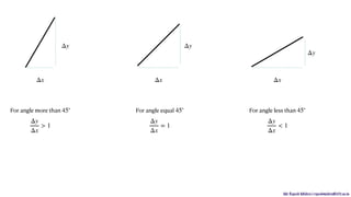
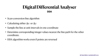
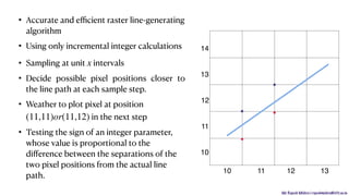
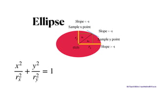
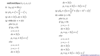
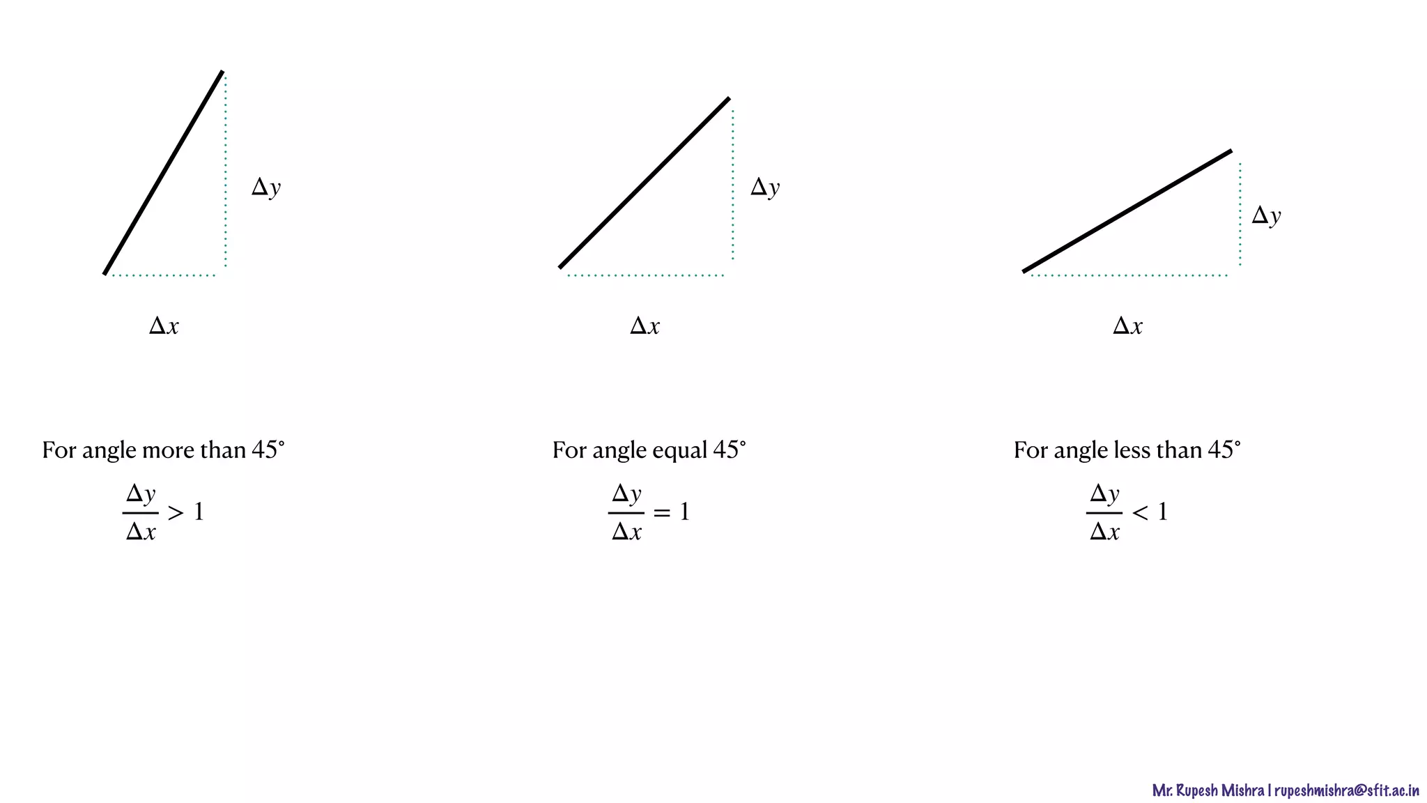
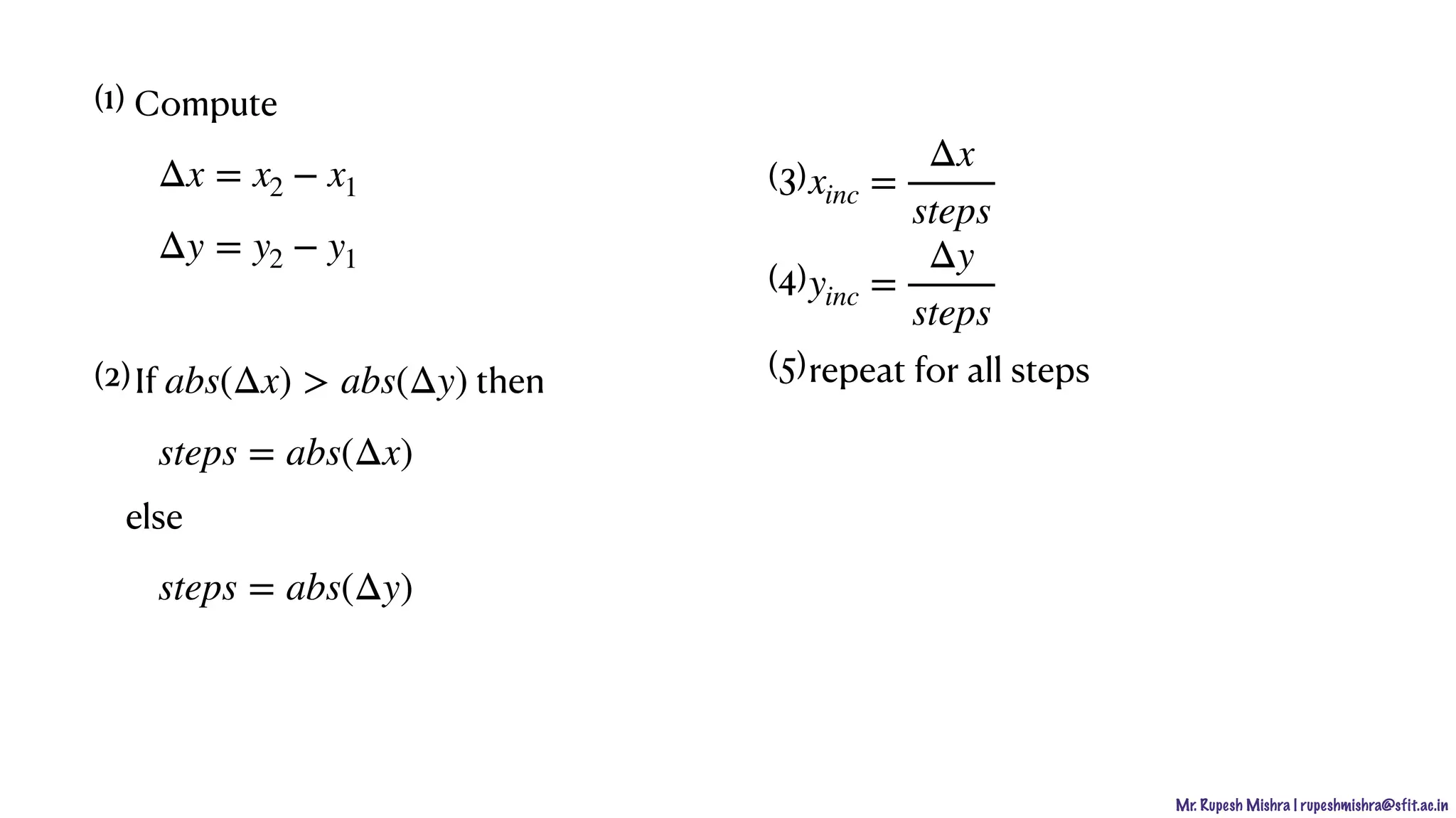
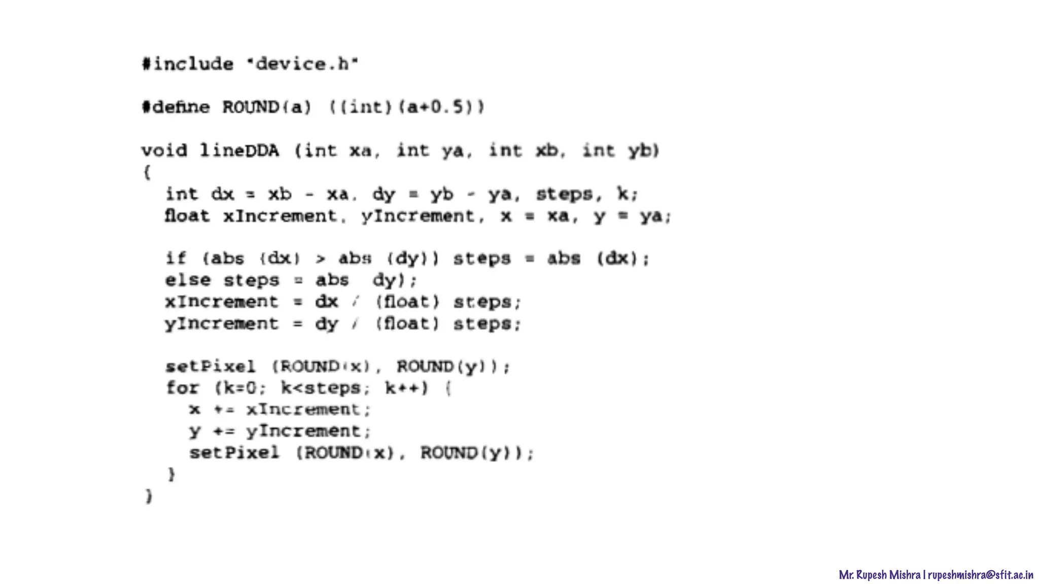
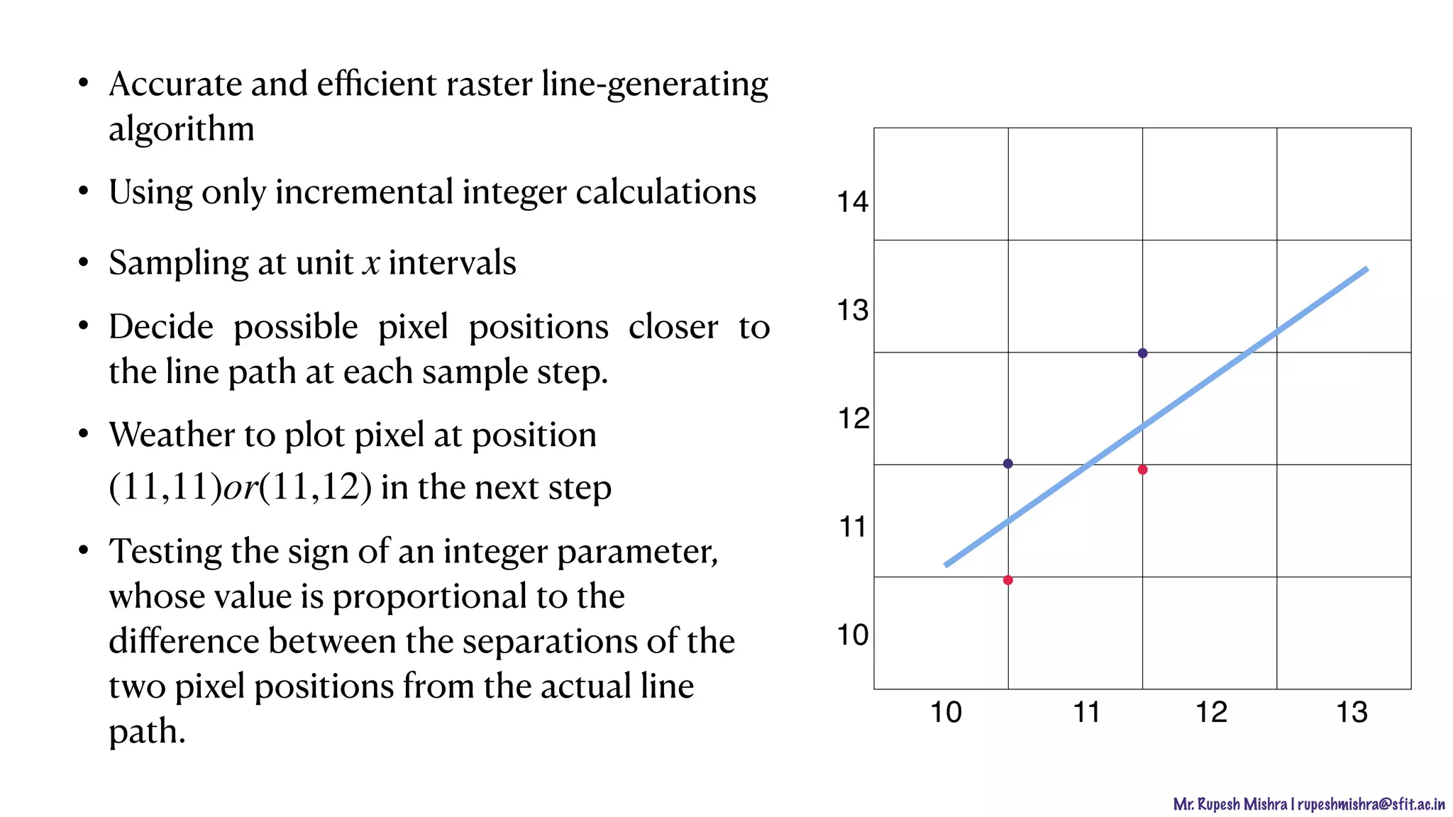
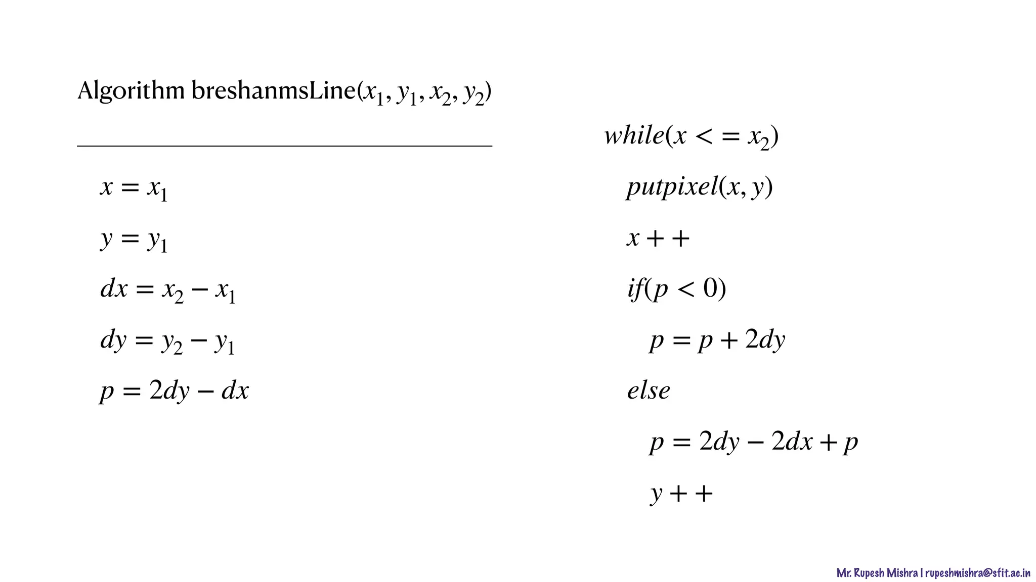
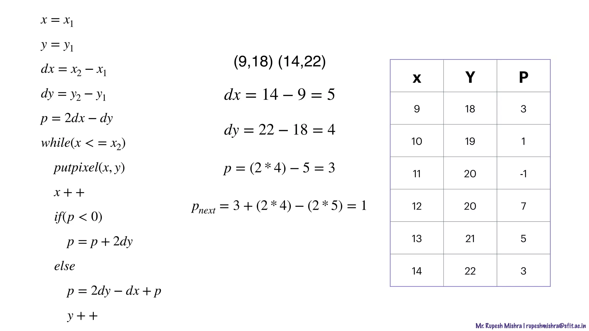
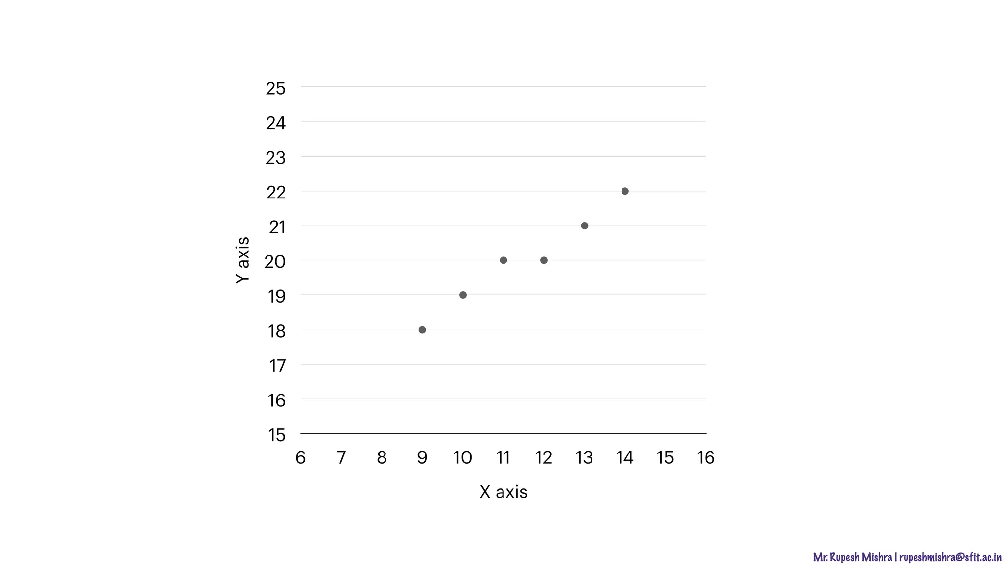
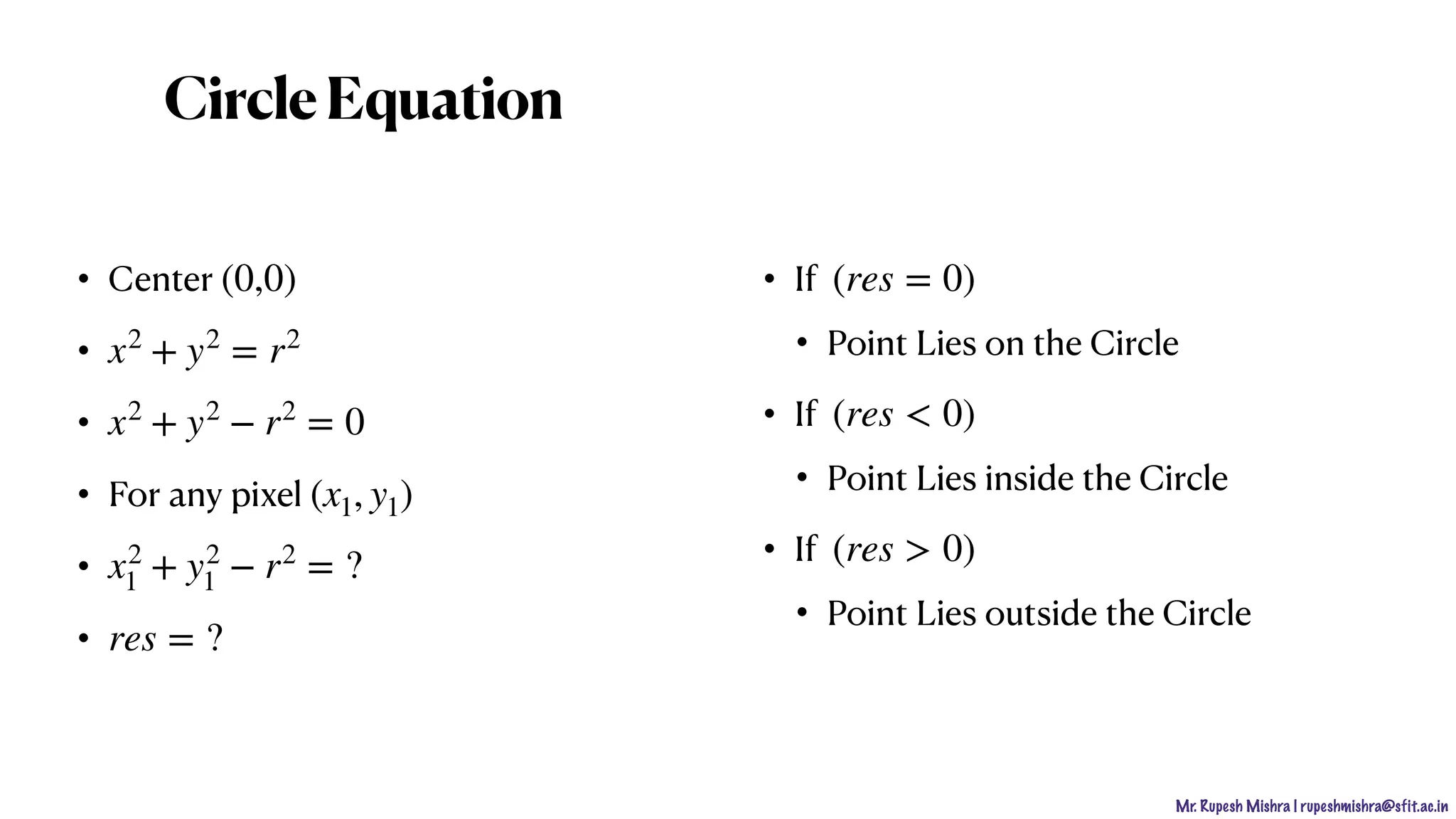
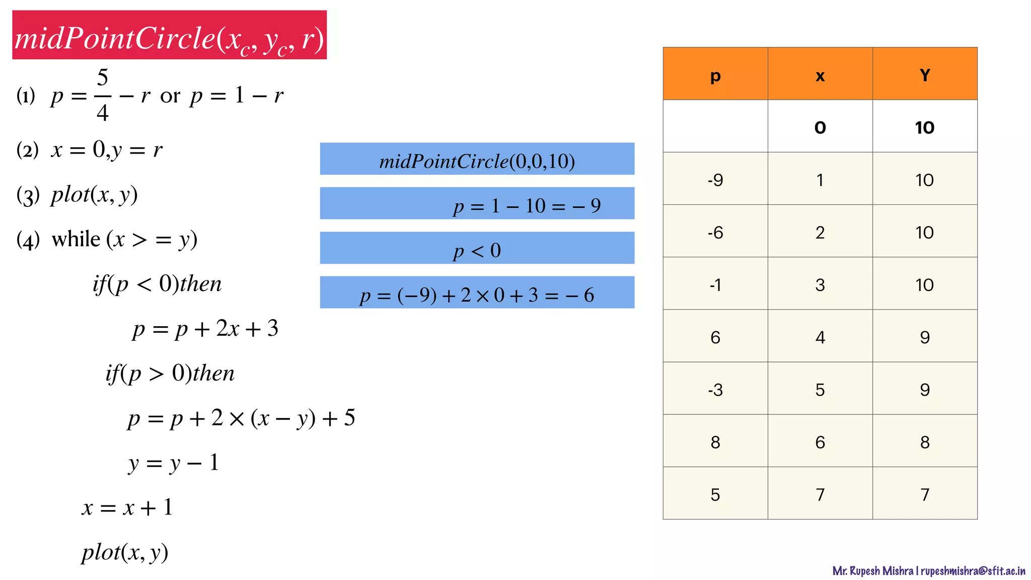
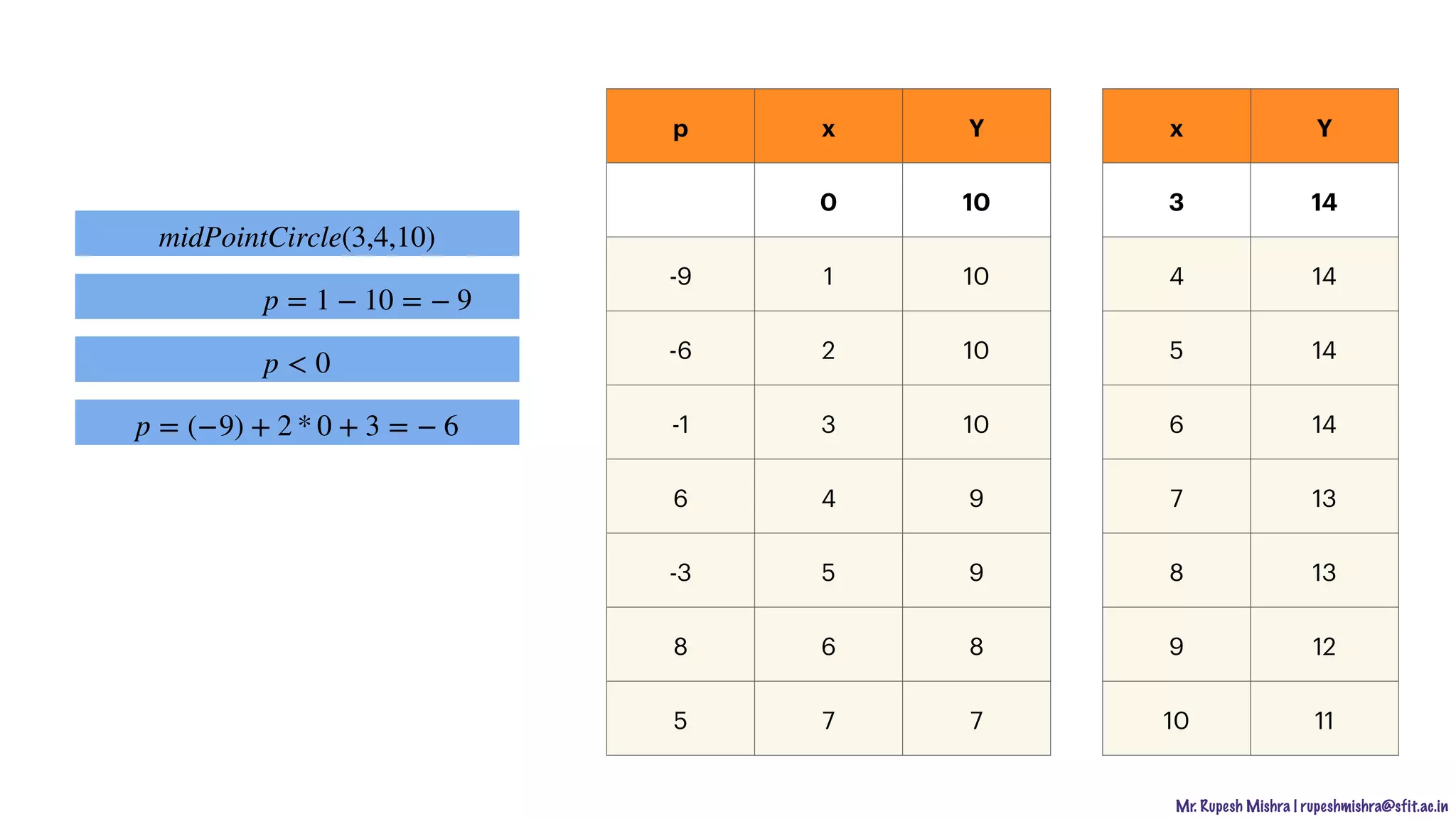
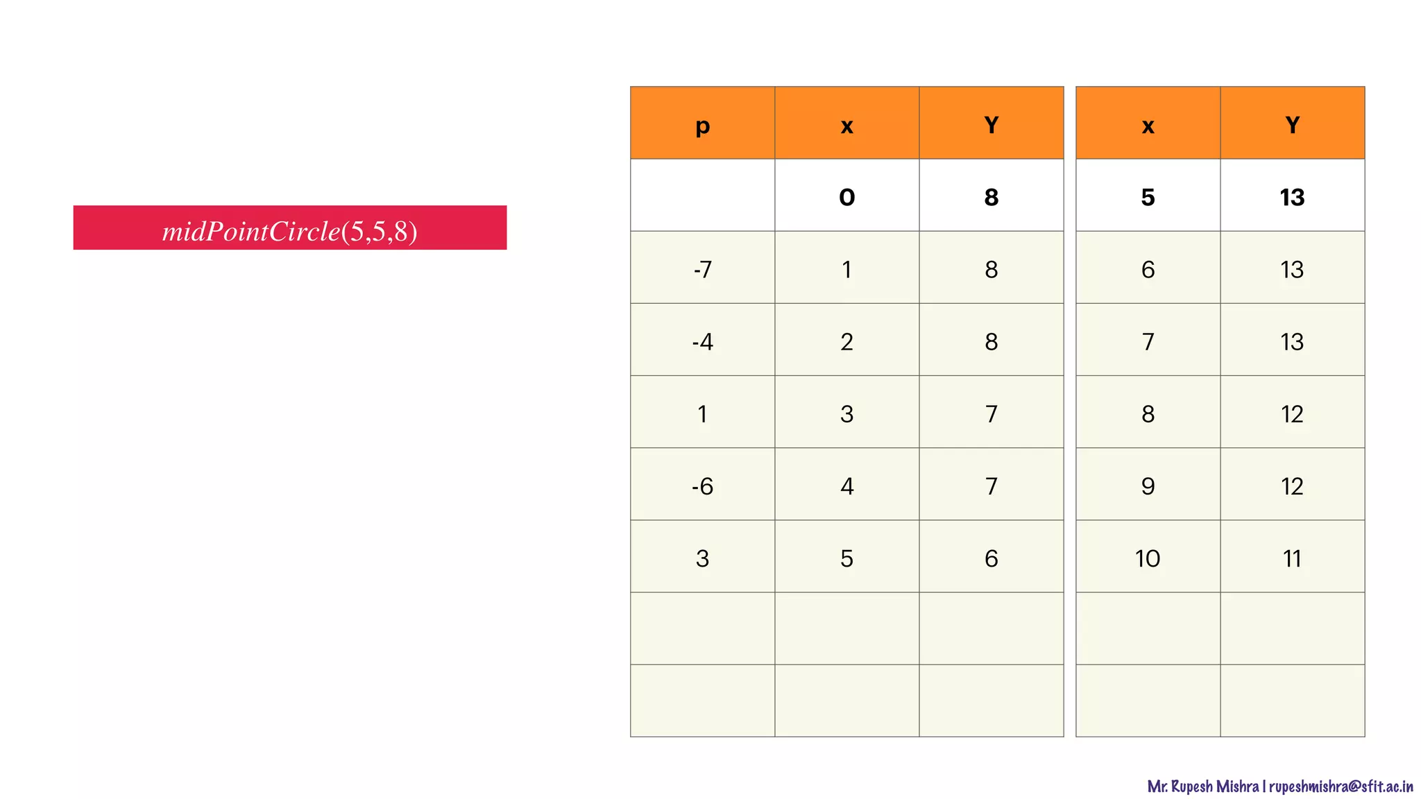
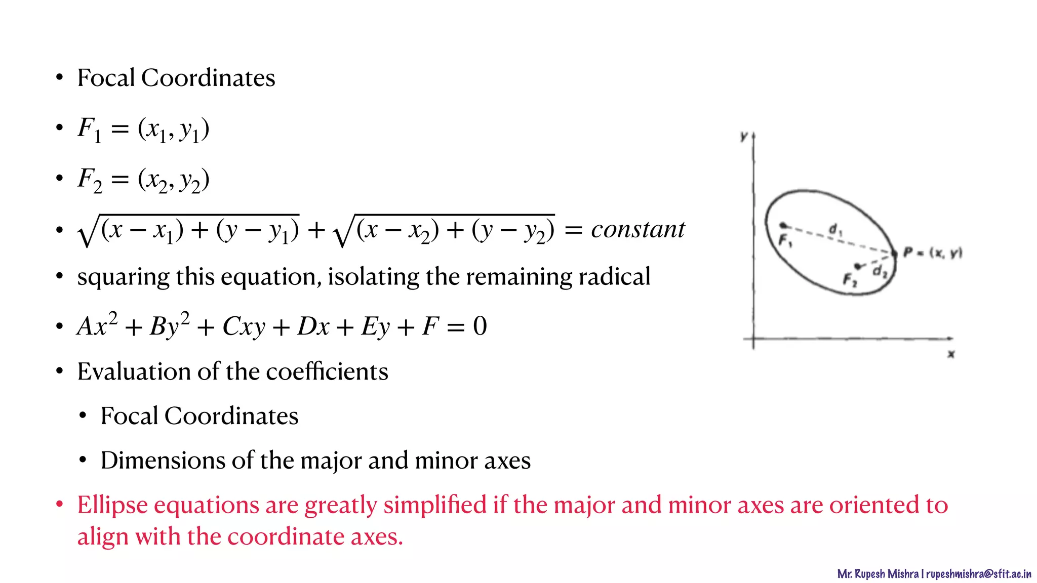
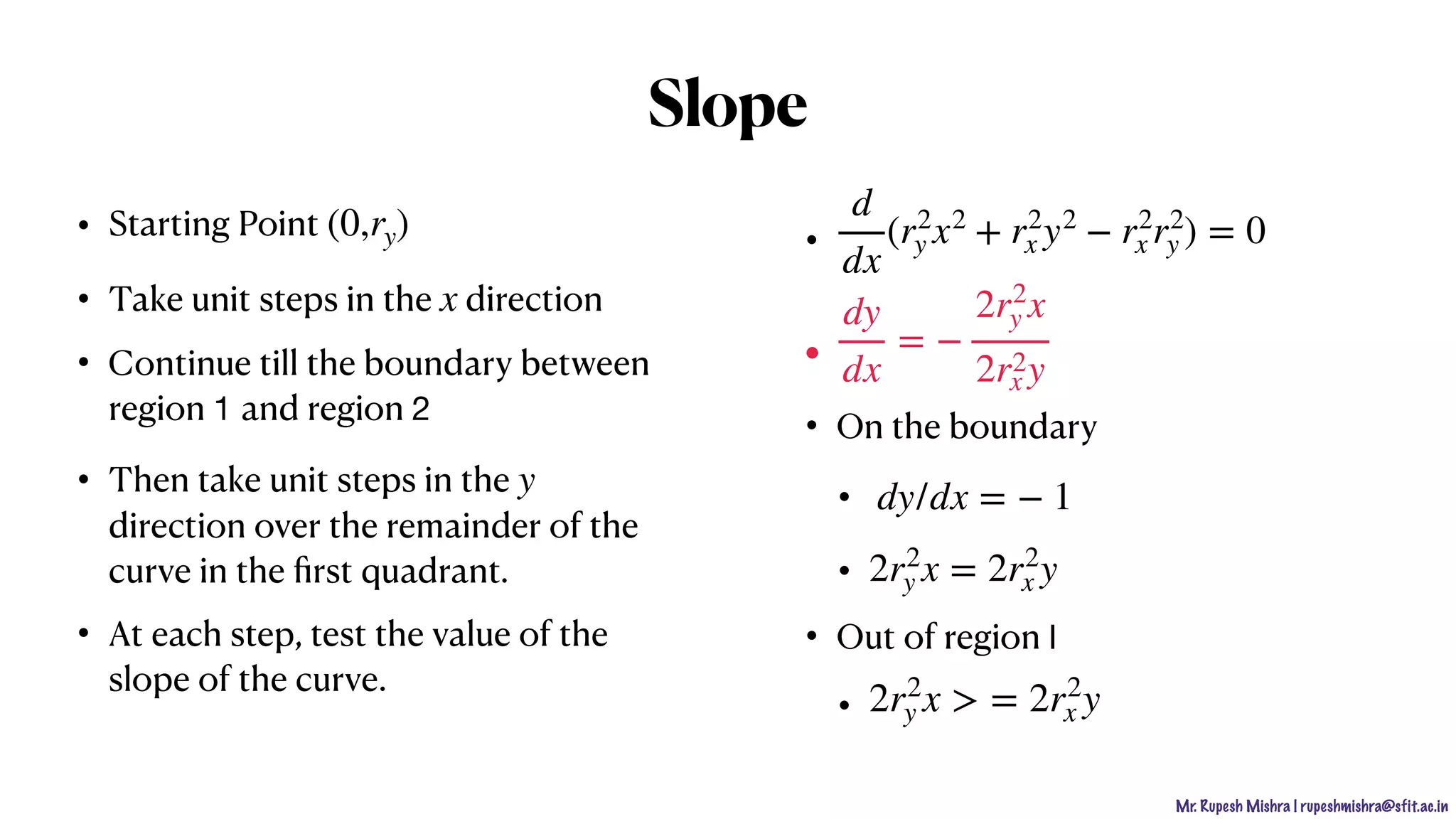
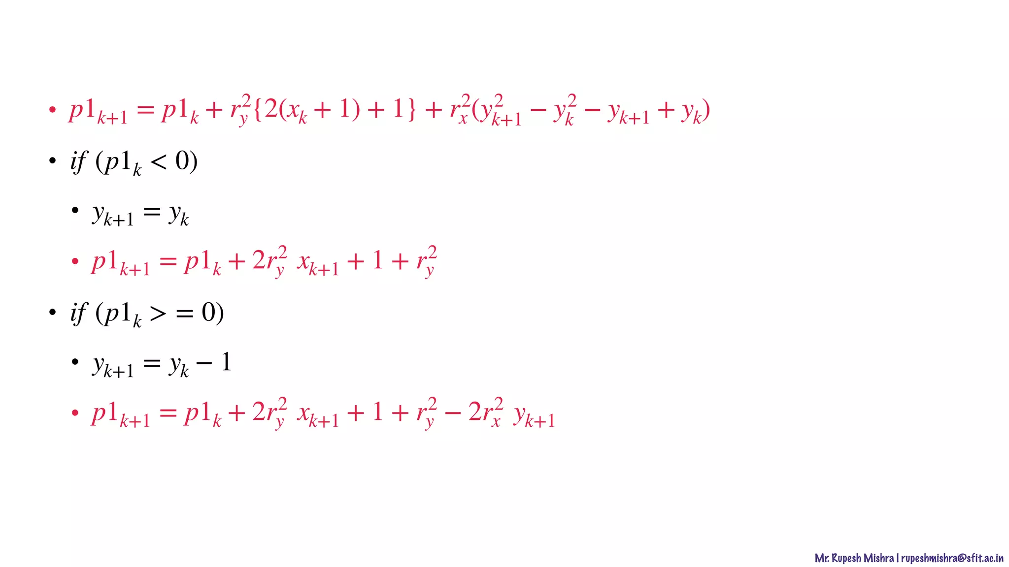
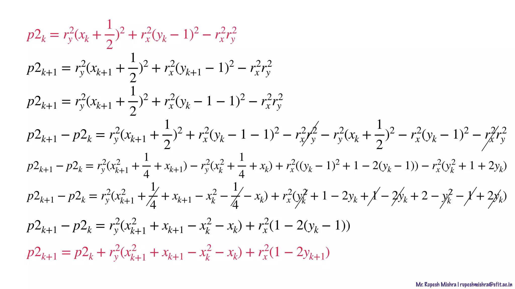
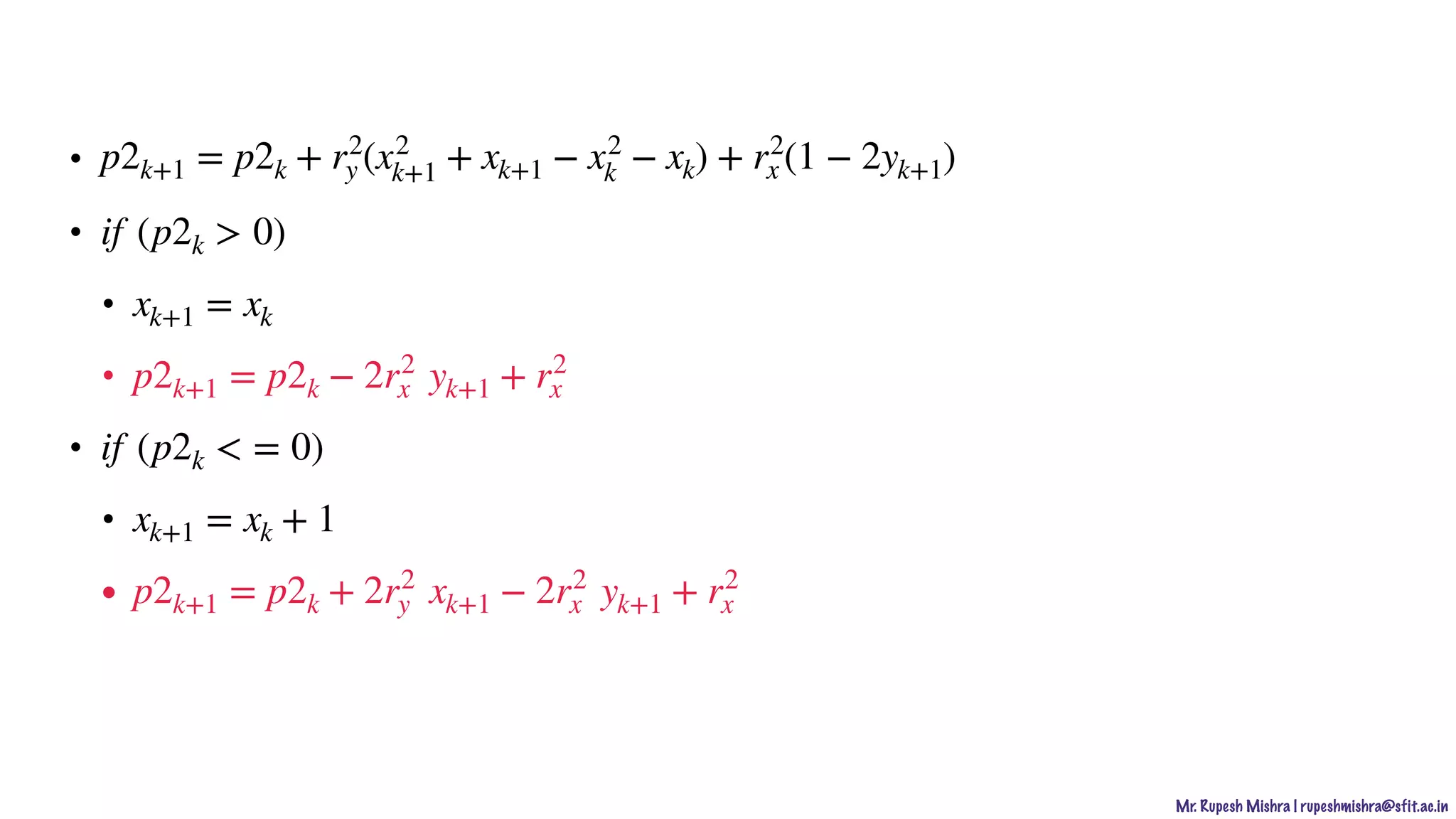
The document describes various output primitives in computer graphics, including points, lines, and circles. It provides details on how each primitive is represented and algorithms for drawing them, such as the digital differential analyzer (DDA) algorithm for lines and the midpoint circle algorithm. Key points covered include how points map to individual pixels, how lines are drawn by plotting discrete points, and how circles can be rendered using either Cartesian equations or parametric equations in polar coordinates.


