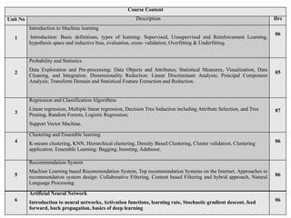
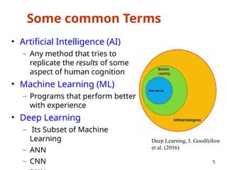
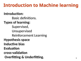
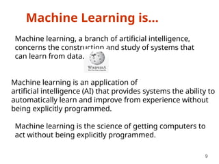
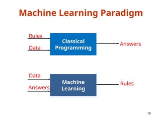
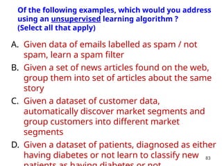
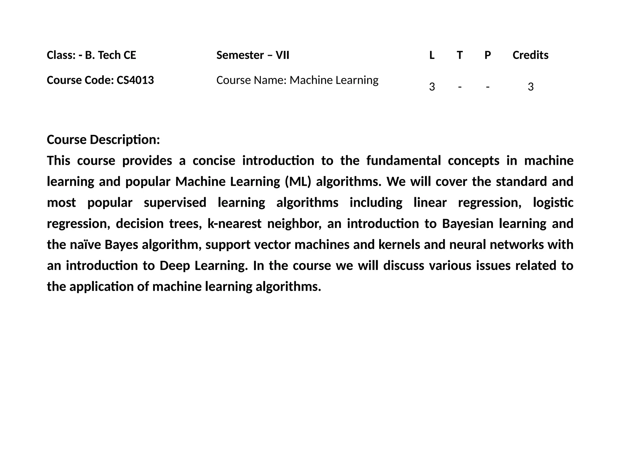
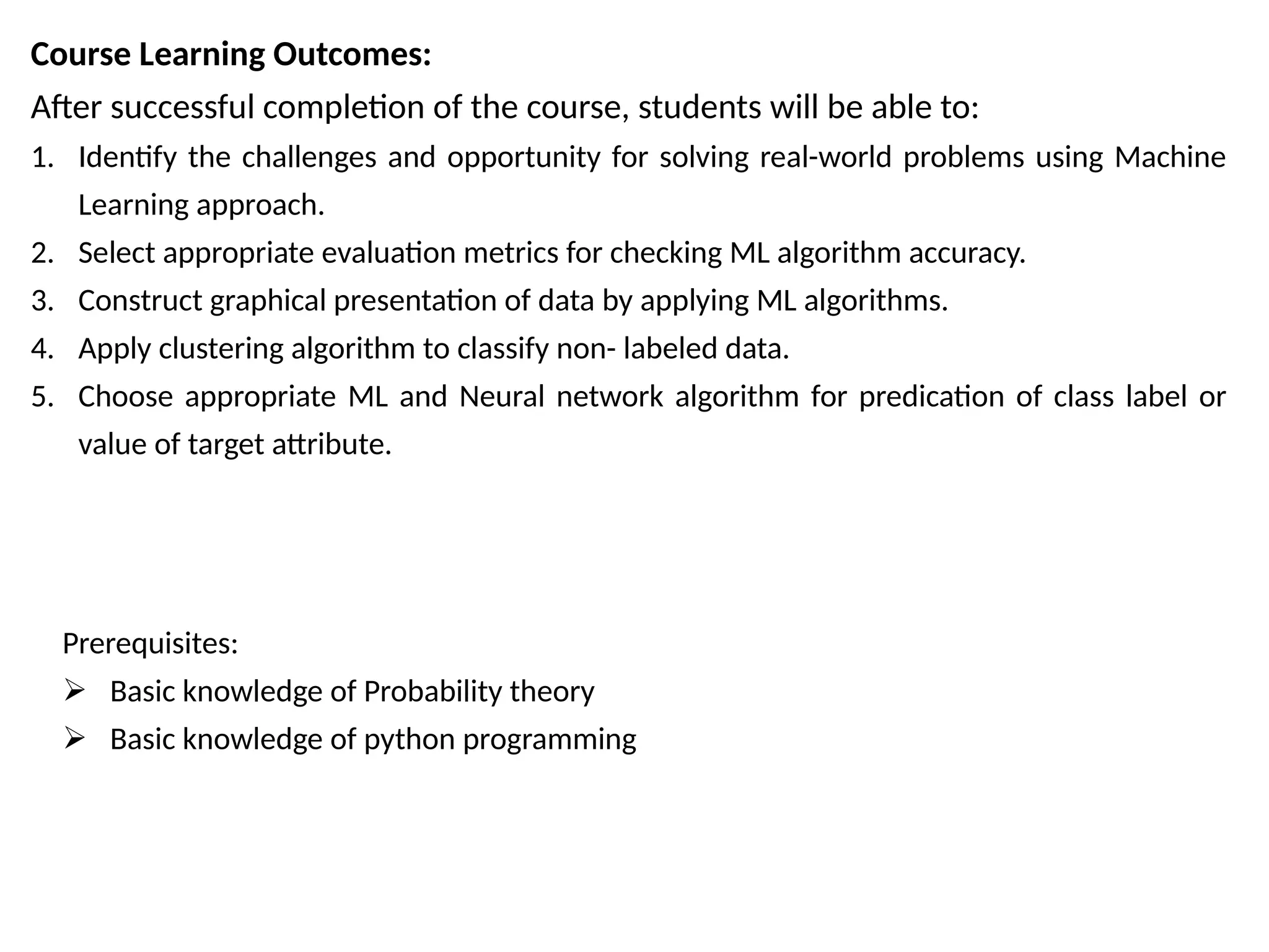
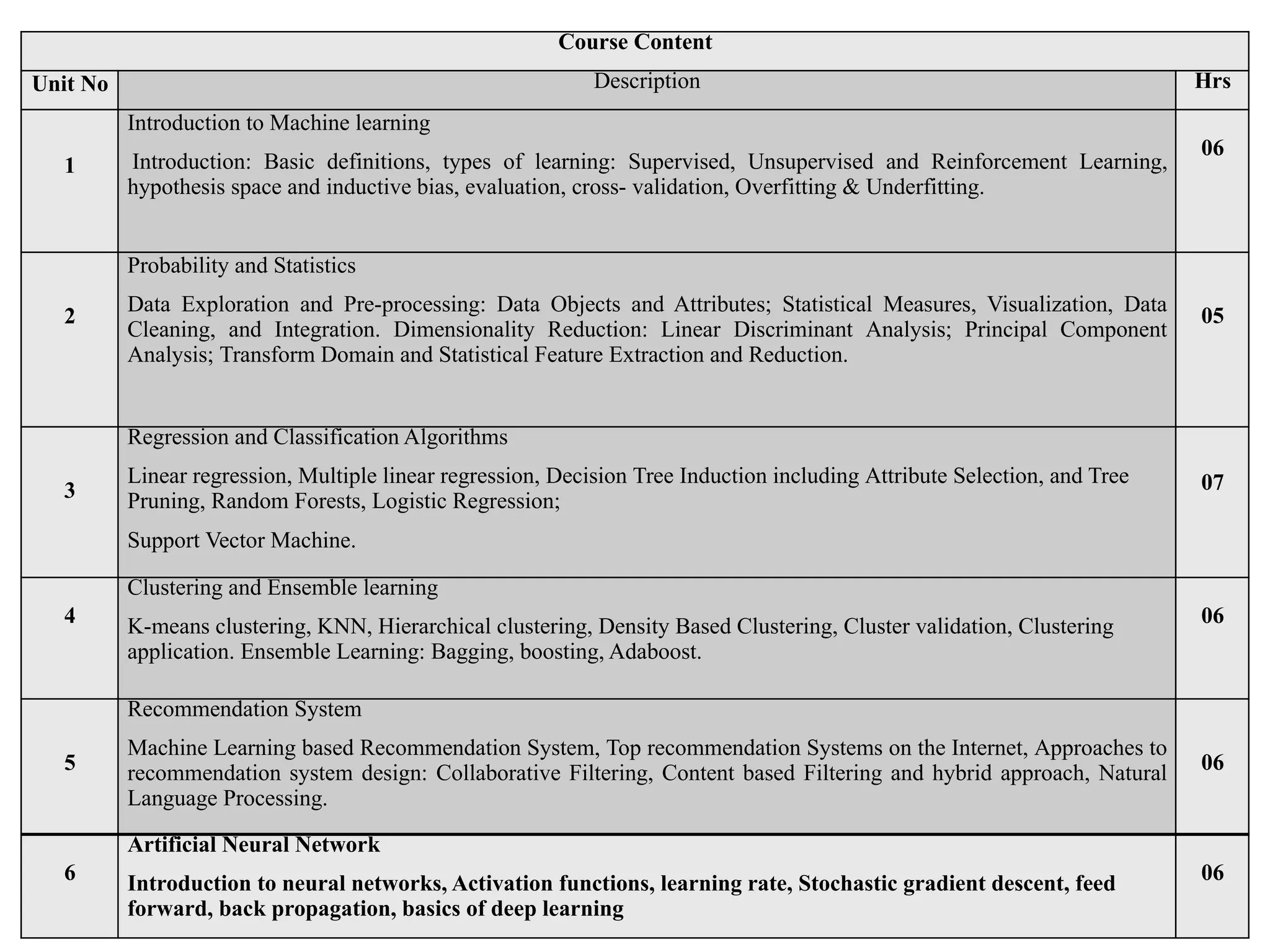
KEMBAR78
Unit - 1 - Introduction of the machine learning | PPTX
Machine Learning
Course Code: CS4013
Course Teacher: Mr. Taranpreet Singh
Class: - B. Tech CE Semester – VII L T P Credits
Course Code: CS4013 Course Name: Machine Learning
3 - - 3
Course Description:
This course provides a concise introduction to the fundamental concepts in machine
learning and popular Machine Learning (ML) algorithms. We will cover the standard and
most popular supervised learning algorithms including linear regression, logistic
regression, decision trees, k-nearest neighbor, an introduction to Bayesian learning and
the naïve Bayes algorithm, support vector machines and kernels and neural networks with
an introduction to Deep Learning. In the course we will discuss various issues related to
the application of machine learning algorithms.
Course Learning Outcomes:
After successful completion of the course, students will be able to:
1. Identify the challenges and opportunity for solving real-world problems using Machine
Learning approach.
2. Select appropriate evaluation metrics for checking ML algorithm accuracy.
3. Construct graphical presentation of data by applying ML algorithms.
4. Apply clustering algorithm to classify non- labeled data.
5. Choose appropriate ML and Neural network algorithm for predication of class label or
value of target attribute.
Prerequisites:
 Basic knowledge of Probability theory
 Basic knowledge of python programming
Course Content
Unit No Description Hrs
1
Introduction to Machine learning
Introduction: Basic definitions, types of learning: Supervised, Unsupervised and Reinforcement Learning,
hypothesis space and inductive bias, evaluation, cross- validation, Overfitting & Underfitting.
06
2
Probability and Statistics
Data Exploration and Pre-processing: Data Objects and Attributes; Statistical Measures, Visualization, Data
Cleaning, and Integration. Dimensionality Reduction: Linear Discriminant Analysis; Principal Component
Analysis; Transform Domain and Statistical Feature Extraction and Reduction.
05
3
Regression and Classification Algorithms
Linear regression, Multiple linear regression, Decision Tree Induction including Attribute Selection, and Tree
Pruning, Random Forests, Logistic Regression;
Support Vector Machine.
07
4
Clustering and Ensemble learning
K-means clustering, KNN, Hierarchical clustering, Density Based Clustering, Cluster validation, Clustering
application. Ensemble Learning: Bagging, boosting, Adaboost.
06
5
Recommendation System
Machine Learning based Recommendation System, Top recommendation Systems on the Internet, Approaches to
recommendation system design: Collaborative Filtering, Content based Filtering and hybrid approach, Natural
Language Processing.
06
6
Artificial Neural Network
Introduction to neural networks, Activation functions, learning rate, Stochastic gradient descent, feed
forward, back propagation, basics of deep learning
06
Some common Terms
• Artificial Intelligence (AI)
– Any method that tries to
replicate the results of some
aspect of human cognition
• Machine Learning (ML)
– Programs that perform better
with experience
• Deep Learning
– Its Subset of Machine
Learning
– ANN
– CNN 5
Deep Learning, I. Goodfellow
et al. (2016)
Introduction to Machine learning
Introduction:
Basic definitions.
Types of learning:
Supervised,
Unsupervised
Reinforcement Learning
Hypothesis space
Inductive bias
Evaluation
cross-validation
Overfitting & Underfitting. 6
What is Machine Learning?
Machine Learning is…
Machine learning, a branch of artificial intelligence,
concerns the construction and study of systems that
can learn from data.
9
Machine learning is an application of
artificial intelligence (AI) that provides systems the ability to
automatically learn and improve from experience without
being explicitly programmed.
Machine learning is the science of getting computers to
act without being explicitly programmed.
Machine Learning Paradigm
10
Classical
Programming
Rules
Data
Answers
Machine
Learning
Data
Answers
Rules
When Machine Learning is
useful?
• When experts are unable to explain their
expertise
– Image recognition
– Speech Recognition
– Driving a car
• When human expertise does not exist
– Hazardous environment – navigation on Mars
• Solution needs to be adapted for particular
cases
– User biometrics
– Patient Specific treatment 11
Machine Learning History
• 1950s
– Samuel’s checker-playing program
• 1960s
– Neural network: Rosenblatt’s
perceptron – delta rule
– Pattern recognition
– Minsky and Papert proved
limitations of perceptron
• 1970s
– Induction of symbolic concepts
– Expert systems
– Natural Language Processing
12
Machine Learning History
• 1980s
– Advanced Decision Trees and Rule Learning
– Resurgence of neural network – MLP – back propagation
algorithm
• 1990s
– Support Vector Machines (SVM)
– Data Mining
– Adaptive agents and web applications
– Text learning
– Reinforcement learning
– Ensembles - Adaboost
– Bayes Network
13
1994: First self driving car made
a road test
1997: Deep Blue beat the world
champion Gary Ksparov in chess
2009: Google built self-driving
car
2011: IBM Watson won Jeopardy
2014: Human Vision surpassed
by ML systems
Why ML is gaining popularity
in recent times?
• New Software and algorithms
– Neural Networks
– Deep Learning
• New Hardware – High Performance Computers
– GPU’s – massive computational power for
computing and online learning
• Cloud Enabled Systems
• Availability of Big Data
16
Definition
• Arthur Samuel (1959):
– Field of study that gives computers the ability to
learn without being explicitly programmed
• Tom Mitchell (1998):
A computer program is said to learn from experience
“E” with respect to some class of tasks “T” and
performance measure “P”, if its performance at tasks
in
“T”, as measured by “P”, improves with experience “E”.
18
Examples
• T: Playing checkers
• P: Percentage of games won against an arbitrary
opponent
• E: Playing practice games against itself
• T: Recognizing hand-written words
• P: Percentage of words correctly classified
• E: Database of human-labeled images of handwritten
words
• T: Categorize email messages as spam or non-spam
• P: Percentage of email messages correctly classified
19
Definition
Hal Daume III:
Machine learning is about predicting the future
based on the past.
Training
Data
learn
model/
predictor
Past
predict
model/
predictor
Future
Testing
Data
Domains and Applications
• Computer Vision
– Say what objects appear in an image
– Convert hand-written digits to characters 0…
9
– Detect where objects appear in an image
21
• Robot Control
– Design autonomous mobile robots that
learn to navigate from their own experience
22
• NLP
– Sentiment analysis: detect if a
product/movie review is positive, negative,
or neutral
– Speech recognition
– Machine translation
23
• Business Intelligence
– Forecasting product sales quantities taking
seasonality and trend in account
– Optimizing product location at a super
market retail outlet
24
Types of Learning
Types of Learning
• Supervised Learning
– X, y (Pre-classified training data)
– Given an observation x, find best label y
• Unsupervised Learning
– X
– Given a set of x’s, cluster them
• Reinforcement Learning
– Determine what to do depends on Rewards
and punishment.
27
Approach
Application
Supervised Learning
33
X y
Input-1 Output-1
Input-2 Output-2
Input-3 Output-3
. .
. .
. .
Input-n Output-n
Learning
Algorithm
Model
New input
x
Output y
Supervised Learning
• Regression
• Classification
34
• A model defined with a set of
parameters.
• Where h() is the model and  are its
parameters
• Regression : y – number
• Classification: y
35
Regression
function
OR
Discriminant
function
)
( 
x
h
y 
Methods under Supervised Learning
• Regression
– Linear Regression
– Logistic Regression
• Classification
– Decision Tree
– Random Forest
– KNN
– SVM
36
Unsupervised Learning
37
X
Input-1
Input-2
Input-3
.
.
.
Input-n
Learning
Algorithm
Clusters
Semi-supervised Learning
38
Reinforcement Learning
• The problem is as
follows: We have an
agent and a reward,
with many hurdles
in between. The
agent is supposed
to find the best
possible path to
reach the reward.
39
Inductive Learning
• Inductive learning or “Prediction”:
– Given examples of a function (X, F(X))
– Predict function F(X) for new examples X
Classification
 F(X) = Discrete
Regression
 F(X) = Continuous
Probability estimation
 F(X) = Probability
40
Terminology – Features
• Instances are described in terms of
features
• Features
– properties that describe each instance
41
Terminology – Feature Space
Feature Space:
Properties that describe the
problem
Credit: Jesse Davis, University of Washington
0.0 1.0 2.0
3.0 4.0 5.0
0.0
1.0
2.0
3.0
42
Terminology
0.0 1.0 2.0
3.0 4.0 5.0
0.0
1.0
2.0
3.0
Sample / Example:
<0.5,2.8,+>
+
+
+ +
+
+
+
+
- -
-
- -
-
-
-
-
- +
+
+
-
-
-
+
+
Credit: Jesse Davis, University of Washington 43
Terminology - Hypothesis
Hypothesis:
Function for labeling examples
+
+
+ +
+
+
+
+
- -
-
- -
-
-
-
-
- +
+
+
-
-
-
+
+ Label: -
Label:+
?
?
?
?
Credit: Jesse Davis, University of Washington
0.0 1.0 2.0
3.0 4.0 5.0
0.0
1.0
2.0
3.0
44
Terminology – Hypothesis Space
Hypothesis Space:
Set of legal hypotheses
+
+
+ +
+
+
+
+
- -
-
- -
-
-
-
-
- +
+
+
-
-
-
+
+
Credit: Jesse Davis, University of Washington
The space of all hypothesis
that can, in principle, be
output by a learning
algorithm.
0.0 1.0 2.0
3.0 4.0 5.0
0.0
1.0
2.0
3.0
45
Hypothesis Space
• A function is represented in terms of
features
• Decide the features
• Define the class of function / language of
the function
 Hypothesis Space
•
46
Representations
• Linear Function
47
• Decision Tree
Representations
• Multivariate Linear Function
48
Representations
• Single Layer
Perceptron
49
• Multi-layer Neural
Network
Terminology
• Training Example <x, y> : Instance x with label y =
f (x)
• Training Data s : Collection of examples observed by
learning algorithm.
• Feature Space / Instance Space X : Set of all possible
objects those can be described by features.
• Concept c : Subset of objects from X (c is unknown).
• Target Function f : Maps each instance x  X to target
label y  Y
50
f : X  Y
Classifier
• Hypothesis h : function that approximates f
• Hypothesis Space H : set of functions we
allow for approximating f
The set of hypotheses that can be
produced, can be restricted further by
specifying a bias
• Input : training set S  X
• Output : hypothesis h  H
51
Size of hypothesis space
• Assume Boolean features
• If there are 4 input features (Boolean),
possible instances = 24
= 16
• Number of Boolean functions possible =
Number of possible subsets of 16 instances =
216
=224
• In general, if N input Boolean features, then
number of possible instances = 2N
and number
of possible functions = 22
N
52
Inductive Bias
• Choosing hypothesis space, needs to make
assumptions
– Experience alone doesn’t allow us to make
conclusions about unseen data instances
• Two types of bias:
– Restriction: Limit the hypothesis space
(e.g., look at rules)
– Preference: Impose ordering on hypothesis
space (e.g., more general, consistent with data)
53
Inductive Learning
• Inducing a general function from training
examples
– To construct hypothesis h to agree with c on
training examples
– A hypothesis is consistent if it agrees with all
training examples
– A hypothesis is said to generalize well if it correctly
predicts the value of y
54
Inductive learning is an ill posed problem : unless we
see all the possible examples, the data is not sufficient
for an inductive learning algorithm to find a unique
solution
Learning as refining the
hypothesis space
• Concept Learning is a task of searching an
hypothesis space of possible representations
looking for the representation(s) that best fits
the data, given the bias
• The tendency to prefer one hypothesis over
another is called a bias
• Occam’s Razor
55
Some more Types of
Inductive Bias
• Minimum description length
• Maximum Margin
56
Evaluation and Cross
Validation
57
Performance Evaluation of
Learning Algorithms
• Few Performance Measures
(Experimental evaluaion)
– Error
– Accuracy
– Precision / Recall
• Typical ways for Sampling Methods
– Train / Test datasets
– K-fold cross validation
58
Evaluating Predictions
•
59
Computation of Error
60
Useful for
regression
problems
•
Criterion function to assess
classifier performance
• Accuracy, error rate
• Other characteristics derived from the
confusion matrix
61
Criterion function to assess
classifier performance
• Accuracy, error rate
– Accuracy is the percent of correct
classifications.
– Error rate = is the percent of incorrect
classifications.
– Accuracy = 1 - Error rate.
62
Confusion matrix, two classes only
TP: Correct acceptance
FP: False alarms
TN: Correct rejections
FN: Misses
Performance measures calculated from the
confusion matrix:
Accuracy = (TN + TP)/total
= (TN + TP)/(TN+TP+FN+FP)
True positive rate, recall, sensitivity =
TP/actual positive = TP / (TP+FN)
True negative rate, specificity =
TN/actual negative = TN / (TN+FP)
Precision, predicted positive value =
TP/predicted positive = TP/(TP+FP)
False positive rate, false alarm =
FP/actual negative = FP/(TN+FP)
= 1 –
specificity 63
Overall, how often
is the classifier
correct?
When it's actually
yes, how often does
it predict yes?
When it's actually
no, how often does
it predict no?
When it predicts
yes, how often is it
correct?
When it's actually
no, how often does
it predict yes?
When it's actually
yes, how often does
it predict no?
Overall, how often
is it wrong?
Confusion matrix : Example
TP: We predicted positive (they have the
disease), and they do have the disease
FP: We predicted yes, but they do not
actually have the disease
TN: We predicted no, and they do not
have the disease
FN: We predicted no, but they actually
do have the disease
Performance measures calculated from
the confusion matrix:
Accuracy = (TN + TP)/total =
(100+50)/165 = 0.91
True positive rate, recall, sensitivity =
TP/actual positive = 100 / 105 = 0.95
True negative rate, specificity =
TN/actual negative = 50 / 60 = 0.83
Precision, predicted positive value =
TP/predicted positive = 100 / 110 = 0.91
False positive rate, false alarm =
FP/actual negative = 10 / 60 = 0.17
False negative rate = FN/actual positive
Two classes : 1. Sample has disease (Positive)
2. No disease
(Negative)
64
Confusion matrix, # of classes > 2
• Example : Predicting true class labels of optical character recognition
for numerals 0-9. There were 100 examples of each number class
available for the evaluation. Empirical performance is given in
percentage.
• The classifier allows the reject option, class label R.
65
Training vs. test data
• Problem: Finite data are available and
have to be used both for training and
testing
– More training data gives better
generalization.
– More test data gives better estimate for the
classification error probability.
–
02/06/2025 66
67
68
Training vs. test data
• Partitioning of available finite set of data to
training / test sets.
– Hold out
– Cross validation
– Bootstrap
–
69
Hold out method
• Given data is randomly partitioned into two
independent sets.
– Training set (e.g., 2/3 of data) for the statistical model
construction, i.e. learning the classifier.
– Test set (e.g., 1/3 of data) is hold out for the accuracy
estimation of the classifier.
• Random sampling is a variation of the hold out method:
– Repeat the hold out k times, the accuracy is estimated as the
average of the accuracies
70
K-fold cross validation
• The training set is randomly
divided into K disjoint sets of
equal size where each part has
roughly the same class
distribution.
• The classifier is trained K times,
each time with a different set
held out as a test set.
• The estimated error is the
mean of these K 71
Stratified Sampling
Leave-one-out
• A special case of K-fold cross validation with K
= n, where n is the total number of samples in
the training multiset.
• n experiments are performed using n 1
−
samples for training and the remaining
sample for testing.
• Computationally expensive.
72
Bootstrap aggregating (bagging)
• Given: training set T with n entries.
• Bootstrap generates k new
datasets Ti each of size n’ <= n by
sampling T with replacement 
some entries can be repeated in Ti.
• The remaining entries that were
not selected for training are used
for testing  This value is likely to
change from fold to fold
• The k statistical models (e.g.,
classifiers, regressors) are learned
using the above k bootstrap
samples.
•
73
• Sampling with replacement to form the training set.
- Improves stability and
accuracy of ML algorithms.
- Reduces variance
- Helps to avoid overfitting.
Three-way data splits
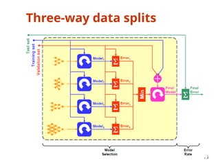
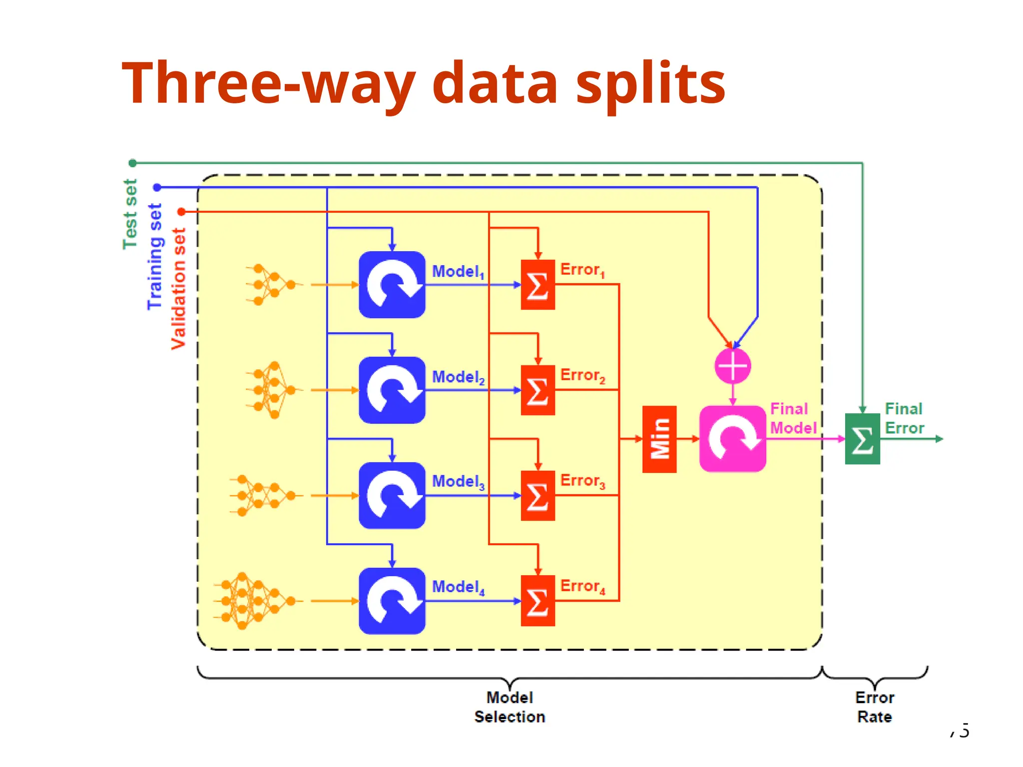
• If model selection and true error estimates are to be
computed simultaneously, the data needs to be divided into
three disjoint sets [Ripley, 1996]
– Training set: a set of examples used for learning: to fit the parameters of the
classifier
– Validation set: a set of examples used to tune the parameters of a classifier
– Test set: a set of examples used only to assess the performance of a fully-
trained classifier
• Why separate test and validation sets?
– The error rate estimate of the final model on validation data will be biased
(smaller than the true error rate) since the validation set is used to select the
final model
– After assessing the final model on the test set, YOU MUST NOT tune the model
any further!
74
Three-way data splits
75
Issues in Machine Learning
• What are good hypothesis spaces ?
• Algorithms that work with the hypothesis spaces
• How to optimize accuracy to future data points ?
• How can we have confidence in the results ?
•
76
QUIZ
80
• Suppose your email program watches which
emails you do or do not mark as spam, based
on that learns how to better filter spam. What
is the task T in this setting ?
A. Classifying emails as spam or not spam
B. Watching you label emails as spam or not spam
C. The number or fraction of emails correctly
classified as spam / not spam
D. None of the above. This is not a machine learnig
problem 81
A computer program is said to learn from experience
E with respect to some task T and some performance
measure P, if its performance on T, as measured by P,
improves with experience E.
Problem 1: You have a large inventory of identical items.
You want to predict how many of these items will sell over
the next 3 months.
Problem 2: You’d like software to examine individual
customer accounts, and for each account decide if it has
been hacked / compromised.
Should you treat these as classification or regression
problem?
A. Treat both as classification problems
B. Treat problem 1 as classification problem, problem 2 as
regression problem
C. Treat problem 1 as regression problem, problem 2 as
classification problem
D. Treat both as regression problems 82
You are running a company, and you want to develop
learning algorithms to address each of two problems
A. Given data of emails labelled as spam / not
spam, learn a spam filter
B. Given a set of news articles found on the web,
group them into set of articles about the same
story
C. Given a dataset of customer data,
automatically discover market segments and
group customers into different market
segments
D. Given a dataset of patients, diagnosed as either
having diabetes or not learn to classify new 83
Of the following examples, which would you address
using an unsupervised learning algorithm ?
(Select all that apply)
84
End of Unit - 1
85

Unit - 1 - Introduction of the machine learning

  • 1.
    Machine Learning Course Code:CS4013 Course Teacher: Mr. Taranpreet Singh
  • 2.
    Class: - B.Tech CE Semester – VII L T P Credits Course Code: CS4013 Course Name: Machine Learning 3 - - 3 Course Description: This course provides a concise introduction to the fundamental concepts in machine learning and popular Machine Learning (ML) algorithms. We will cover the standard and most popular supervised learning algorithms including linear regression, logistic regression, decision trees, k-nearest neighbor, an introduction to Bayesian learning and the naïve Bayes algorithm, support vector machines and kernels and neural networks with an introduction to Deep Learning. In the course we will discuss various issues related to the application of machine learning algorithms.
  • 3.
    Course Learning Outcomes: Aftersuccessful completion of the course, students will be able to: 1. Identify the challenges and opportunity for solving real-world problems using Machine Learning approach. 2. Select appropriate evaluation metrics for checking ML algorithm accuracy. 3. Construct graphical presentation of data by applying ML algorithms. 4. Apply clustering algorithm to classify non- labeled data. 5. Choose appropriate ML and Neural network algorithm for predication of class label or value of target attribute. Prerequisites:  Basic knowledge of Probability theory  Basic knowledge of python programming
  • 4.
    Course Content Unit NoDescription Hrs 1 Introduction to Machine learning Introduction: Basic definitions, types of learning: Supervised, Unsupervised and Reinforcement Learning, hypothesis space and inductive bias, evaluation, cross- validation, Overfitting & Underfitting. 06 2 Probability and Statistics Data Exploration and Pre-processing: Data Objects and Attributes; Statistical Measures, Visualization, Data Cleaning, and Integration. Dimensionality Reduction: Linear Discriminant Analysis; Principal Component Analysis; Transform Domain and Statistical Feature Extraction and Reduction. 05 3 Regression and Classification Algorithms Linear regression, Multiple linear regression, Decision Tree Induction including Attribute Selection, and Tree Pruning, Random Forests, Logistic Regression; Support Vector Machine. 07 4 Clustering and Ensemble learning K-means clustering, KNN, Hierarchical clustering, Density Based Clustering, Cluster validation, Clustering application. Ensemble Learning: Bagging, boosting, Adaboost. 06 5 Recommendation System Machine Learning based Recommendation System, Top recommendation Systems on the Internet, Approaches to recommendation system design: Collaborative Filtering, Content based Filtering and hybrid approach, Natural Language Processing. 06 6 Artificial Neural Network Introduction to neural networks, Activation functions, learning rate, Stochastic gradient descent, feed forward, back propagation, basics of deep learning 06
  • 5.
    Some common Terms •Artificial Intelligence (AI) – Any method that tries to replicate the results of some aspect of human cognition • Machine Learning (ML) – Programs that perform better with experience • Deep Learning – Its Subset of Machine Learning – ANN – CNN 5 Deep Learning, I. Goodfellow et al. (2016)
  • 6.
    Introduction to Machinelearning Introduction: Basic definitions. Types of learning: Supervised, Unsupervised Reinforcement Learning Hypothesis space Inductive bias Evaluation cross-validation Overfitting & Underfitting. 6
  • 7.
    What is MachineLearning?
  • 8.
    Machine Learning is… Machinelearning, a branch of artificial intelligence, concerns the construction and study of systems that can learn from data. 9 Machine learning is an application of artificial intelligence (AI) that provides systems the ability to automatically learn and improve from experience without being explicitly programmed. Machine learning is the science of getting computers to act without being explicitly programmed.
  • 9.
  • 10.
    When Machine Learningis useful? • When experts are unable to explain their expertise – Image recognition – Speech Recognition – Driving a car • When human expertise does not exist – Hazardous environment – navigation on Mars • Solution needs to be adapted for particular cases – User biometrics – Patient Specific treatment 11
  • 11.
    Machine Learning History •1950s – Samuel’s checker-playing program • 1960s – Neural network: Rosenblatt’s perceptron – delta rule – Pattern recognition – Minsky and Papert proved limitations of perceptron • 1970s – Induction of symbolic concepts – Expert systems – Natural Language Processing 12
  • 12.
    Machine Learning History •1980s – Advanced Decision Trees and Rule Learning – Resurgence of neural network – MLP – back propagation algorithm • 1990s – Support Vector Machines (SVM) – Data Mining – Adaptive agents and web applications – Text learning – Reinforcement learning – Ensembles - Adaboost – Bayes Network 13 1994: First self driving car made a road test 1997: Deep Blue beat the world champion Gary Ksparov in chess 2009: Google built self-driving car 2011: IBM Watson won Jeopardy 2014: Human Vision surpassed by ML systems
  • 15.
    Why ML isgaining popularity in recent times? • New Software and algorithms – Neural Networks – Deep Learning • New Hardware – High Performance Computers – GPU’s – massive computational power for computing and online learning • Cloud Enabled Systems • Availability of Big Data 16
  • 16.
    Definition • Arthur Samuel(1959): – Field of study that gives computers the ability to learn without being explicitly programmed • Tom Mitchell (1998): A computer program is said to learn from experience “E” with respect to some class of tasks “T” and performance measure “P”, if its performance at tasks in “T”, as measured by “P”, improves with experience “E”. 18
  • 17.
    Examples • T: Playingcheckers • P: Percentage of games won against an arbitrary opponent • E: Playing practice games against itself • T: Recognizing hand-written words • P: Percentage of words correctly classified • E: Database of human-labeled images of handwritten words • T: Categorize email messages as spam or non-spam • P: Percentage of email messages correctly classified 19
  • 18.
    Definition Hal Daume III: Machinelearning is about predicting the future based on the past. Training Data learn model/ predictor Past predict model/ predictor Future Testing Data
  • 19.
    Domains and Applications •Computer Vision – Say what objects appear in an image – Convert hand-written digits to characters 0… 9 – Detect where objects appear in an image 21
  • 20.
    • Robot Control –Design autonomous mobile robots that learn to navigate from their own experience 22
  • 21.
    • NLP – Sentimentanalysis: detect if a product/movie review is positive, negative, or neutral – Speech recognition – Machine translation 23
  • 22.
    • Business Intelligence –Forecasting product sales quantities taking seasonality and trend in account – Optimizing product location at a super market retail outlet 24
  • 24.
  • 25.
    Types of Learning •Supervised Learning – X, y (Pre-classified training data) – Given an observation x, find best label y • Unsupervised Learning – X – Given a set of x’s, cluster them • Reinforcement Learning – Determine what to do depends on Rewards and punishment. 27
  • 28.
  • 30.
  • 31.
    Supervised Learning 33 X y Input-1Output-1 Input-2 Output-2 Input-3 Output-3 . . . . . . Input-n Output-n Learning Algorithm Model New input x Output y
  • 32.
  • 33.
    • A modeldefined with a set of parameters. • Where h() is the model and  are its parameters • Regression : y – number • Classification: y 35 Regression function OR Discriminant function ) (  x h y 
  • 34.
    Methods under SupervisedLearning • Regression – Linear Regression – Logistic Regression • Classification – Decision Tree – Random Forest – KNN – SVM 36
  • 35.
  • 36.
  • 37.
    Reinforcement Learning • Theproblem is as follows: We have an agent and a reward, with many hurdles in between. The agent is supposed to find the best possible path to reach the reward. 39
  • 38.
    Inductive Learning • Inductivelearning or “Prediction”: – Given examples of a function (X, F(X)) – Predict function F(X) for new examples X Classification  F(X) = Discrete Regression  F(X) = Continuous Probability estimation  F(X) = Probability 40
  • 39.
    Terminology – Features •Instances are described in terms of features • Features – properties that describe each instance 41
  • 40.
    Terminology – FeatureSpace Feature Space: Properties that describe the problem Credit: Jesse Davis, University of Washington 0.0 1.0 2.0 3.0 4.0 5.0 0.0 1.0 2.0 3.0 42
  • 41.
    Terminology 0.0 1.0 2.0 3.04.0 5.0 0.0 1.0 2.0 3.0 Sample / Example: <0.5,2.8,+> + + + + + + + + - - - - - - - - - - + + + - - - + + Credit: Jesse Davis, University of Washington 43
  • 42.
    Terminology - Hypothesis Hypothesis: Functionfor labeling examples + + + + + + + + - - - - - - - - - - + + + - - - + + Label: - Label:+ ? ? ? ? Credit: Jesse Davis, University of Washington 0.0 1.0 2.0 3.0 4.0 5.0 0.0 1.0 2.0 3.0 44
  • 43.
    Terminology – HypothesisSpace Hypothesis Space: Set of legal hypotheses + + + + + + + + - - - - - - - - - - + + + - - - + + Credit: Jesse Davis, University of Washington The space of all hypothesis that can, in principle, be output by a learning algorithm. 0.0 1.0 2.0 3.0 4.0 5.0 0.0 1.0 2.0 3.0 45
  • 44.
    Hypothesis Space • Afunction is represented in terms of features • Decide the features • Define the class of function / language of the function  Hypothesis Space • 46
  • 45.
  • 46.
  • 47.
  • 48.
    Terminology • Training Example<x, y> : Instance x with label y = f (x) • Training Data s : Collection of examples observed by learning algorithm. • Feature Space / Instance Space X : Set of all possible objects those can be described by features. • Concept c : Subset of objects from X (c is unknown). • Target Function f : Maps each instance x  X to target label y  Y 50 f : X  Y
  • 49.
    Classifier • Hypothesis h: function that approximates f • Hypothesis Space H : set of functions we allow for approximating f The set of hypotheses that can be produced, can be restricted further by specifying a bias • Input : training set S  X • Output : hypothesis h  H 51
  • 50.
    Size of hypothesisspace • Assume Boolean features • If there are 4 input features (Boolean), possible instances = 24 = 16 • Number of Boolean functions possible = Number of possible subsets of 16 instances = 216 =224 • In general, if N input Boolean features, then number of possible instances = 2N and number of possible functions = 22 N 52
  • 51.
    Inductive Bias • Choosinghypothesis space, needs to make assumptions – Experience alone doesn’t allow us to make conclusions about unseen data instances • Two types of bias: – Restriction: Limit the hypothesis space (e.g., look at rules) – Preference: Impose ordering on hypothesis space (e.g., more general, consistent with data) 53
  • 52.
    Inductive Learning • Inducinga general function from training examples – To construct hypothesis h to agree with c on training examples – A hypothesis is consistent if it agrees with all training examples – A hypothesis is said to generalize well if it correctly predicts the value of y 54 Inductive learning is an ill posed problem : unless we see all the possible examples, the data is not sufficient for an inductive learning algorithm to find a unique solution
  • 53.
    Learning as refiningthe hypothesis space • Concept Learning is a task of searching an hypothesis space of possible representations looking for the representation(s) that best fits the data, given the bias • The tendency to prefer one hypothesis over another is called a bias • Occam’s Razor 55
  • 54.
    Some more Typesof Inductive Bias • Minimum description length • Maximum Margin 56
  • 55.
  • 56.
    Performance Evaluation of LearningAlgorithms • Few Performance Measures (Experimental evaluaion) – Error – Accuracy – Precision / Recall • Typical ways for Sampling Methods – Train / Test datasets – K-fold cross validation 58
  • 57.
  • 58.
    Computation of Error 60 Usefulfor regression problems •
  • 59.
    Criterion function toassess classifier performance • Accuracy, error rate • Other characteristics derived from the confusion matrix 61
  • 60.
    Criterion function toassess classifier performance • Accuracy, error rate – Accuracy is the percent of correct classifications. – Error rate = is the percent of incorrect classifications. – Accuracy = 1 - Error rate. 62
  • 61.
    Confusion matrix, twoclasses only TP: Correct acceptance FP: False alarms TN: Correct rejections FN: Misses Performance measures calculated from the confusion matrix: Accuracy = (TN + TP)/total = (TN + TP)/(TN+TP+FN+FP) True positive rate, recall, sensitivity = TP/actual positive = TP / (TP+FN) True negative rate, specificity = TN/actual negative = TN / (TN+FP) Precision, predicted positive value = TP/predicted positive = TP/(TP+FP) False positive rate, false alarm = FP/actual negative = FP/(TN+FP) = 1 – specificity 63 Overall, how often is the classifier correct? When it's actually yes, how often does it predict yes? When it's actually no, how often does it predict no? When it predicts yes, how often is it correct? When it's actually no, how often does it predict yes? When it's actually yes, how often does it predict no? Overall, how often is it wrong?
  • 62.
    Confusion matrix :Example TP: We predicted positive (they have the disease), and they do have the disease FP: We predicted yes, but they do not actually have the disease TN: We predicted no, and they do not have the disease FN: We predicted no, but they actually do have the disease Performance measures calculated from the confusion matrix: Accuracy = (TN + TP)/total = (100+50)/165 = 0.91 True positive rate, recall, sensitivity = TP/actual positive = 100 / 105 = 0.95 True negative rate, specificity = TN/actual negative = 50 / 60 = 0.83 Precision, predicted positive value = TP/predicted positive = 100 / 110 = 0.91 False positive rate, false alarm = FP/actual negative = 10 / 60 = 0.17 False negative rate = FN/actual positive Two classes : 1. Sample has disease (Positive) 2. No disease (Negative) 64
  • 63.
    Confusion matrix, #of classes > 2 • Example : Predicting true class labels of optical character recognition for numerals 0-9. There were 100 examples of each number class available for the evaluation. Empirical performance is given in percentage. • The classifier allows the reject option, class label R. 65
  • 64.
    Training vs. testdata • Problem: Finite data are available and have to be used both for training and testing – More training data gives better generalization. – More test data gives better estimate for the classification error probability. – 02/06/2025 66
  • 65.
  • 66.
  • 67.
    Training vs. testdata • Partitioning of available finite set of data to training / test sets. – Hold out – Cross validation – Bootstrap – 69
  • 68.
    Hold out method •Given data is randomly partitioned into two independent sets. – Training set (e.g., 2/3 of data) for the statistical model construction, i.e. learning the classifier. – Test set (e.g., 1/3 of data) is hold out for the accuracy estimation of the classifier. • Random sampling is a variation of the hold out method: – Repeat the hold out k times, the accuracy is estimated as the average of the accuracies 70
  • 69.
    K-fold cross validation •The training set is randomly divided into K disjoint sets of equal size where each part has roughly the same class distribution. • The classifier is trained K times, each time with a different set held out as a test set. • The estimated error is the mean of these K 71 Stratified Sampling
  • 70.
    Leave-one-out • A specialcase of K-fold cross validation with K = n, where n is the total number of samples in the training multiset. • n experiments are performed using n 1 − samples for training and the remaining sample for testing. • Computationally expensive. 72
  • 71.
    Bootstrap aggregating (bagging) •Given: training set T with n entries. • Bootstrap generates k new datasets Ti each of size n’ <= n by sampling T with replacement  some entries can be repeated in Ti. • The remaining entries that were not selected for training are used for testing  This value is likely to change from fold to fold • The k statistical models (e.g., classifiers, regressors) are learned using the above k bootstrap samples. • 73 • Sampling with replacement to form the training set. - Improves stability and accuracy of ML algorithms. - Reduces variance - Helps to avoid overfitting.
  • 72.
    Three-way data splits •If model selection and true error estimates are to be computed simultaneously, the data needs to be divided into three disjoint sets [Ripley, 1996] – Training set: a set of examples used for learning: to fit the parameters of the classifier – Validation set: a set of examples used to tune the parameters of a classifier – Test set: a set of examples used only to assess the performance of a fully- trained classifier • Why separate test and validation sets? – The error rate estimate of the final model on validation data will be biased (smaller than the true error rate) since the validation set is used to select the final model – After assessing the final model on the test set, YOU MUST NOT tune the model any further! 74
  • 73.
  • 74.
    Issues in MachineLearning • What are good hypothesis spaces ? • Algorithms that work with the hypothesis spaces • How to optimize accuracy to future data points ? • How can we have confidence in the results ? • 76
  • 75.
  • 76.
    • Suppose youremail program watches which emails you do or do not mark as spam, based on that learns how to better filter spam. What is the task T in this setting ? A. Classifying emails as spam or not spam B. Watching you label emails as spam or not spam C. The number or fraction of emails correctly classified as spam / not spam D. None of the above. This is not a machine learnig problem 81 A computer program is said to learn from experience E with respect to some task T and some performance measure P, if its performance on T, as measured by P, improves with experience E.
  • 77.
    Problem 1: Youhave a large inventory of identical items. You want to predict how many of these items will sell over the next 3 months. Problem 2: You’d like software to examine individual customer accounts, and for each account decide if it has been hacked / compromised. Should you treat these as classification or regression problem? A. Treat both as classification problems B. Treat problem 1 as classification problem, problem 2 as regression problem C. Treat problem 1 as regression problem, problem 2 as classification problem D. Treat both as regression problems 82 You are running a company, and you want to develop learning algorithms to address each of two problems
  • 78.
    A. Given dataof emails labelled as spam / not spam, learn a spam filter B. Given a set of news articles found on the web, group them into set of articles about the same story C. Given a dataset of customer data, automatically discover market segments and group customers into different market segments D. Given a dataset of patients, diagnosed as either having diabetes or not learn to classify new 83 Of the following examples, which would you address using an unsupervised learning algorithm ? (Select all that apply)
  • 79.
  • 80.

Editor's Notes

  • #5 Frequently, we come across few common terms. One is the term of artificial intelligence. Artificial intelligence is a very broad term, it simply means animator that tries to replicate the results of some aspect of human cognition. The reason the word results is being emphasized, is because we might not actually replicate the processes themselves but only the results. So, if somebody is playing chess, somebody is driving car, all you want to do is to make sure that the final output is the same, whether it is a machine or whether it is a human being. As against this, machine learning is a specific term, that means programs that actually perform better as your experience grows. What is meant by experience is something that we will discuss a little bit later. At what it means is if you have, let us say Calculator, the calculator is not getting better. You know, as you ask it to do multiplications again and again and again, but if a human being is there, the person might actually get more accurate or faster as they do multiplications for a while. So, machine learning, if suppose to replicate this process which is as experience in a field grows, whether it is spam detection, or whether it is vision or anything of that sort. Machine learning if the set of algorithms which actually gets better. Artificial intelligence might or might not actually get better with experience. You would have also heard the term neural networks or artificial neural networks, there are type of machine learning algorithm. And most commonly, you would have heard a term Deep Learning, which is a certain type of artificial neural network. Nowadays it is being used in a broader sense, but more technically, all it means is a neural network with a bunch of layers, which we will see later.
  • #10 In a classical programming thing, you have certain rules and your certain data, it is processed by the program and gives answers. For example if you have classical programming approach to spam detection, you would have certain rules. For example if there are too many caps or if the email talks about money and puts a dollar in the middle, something of that sort, those would be the rule. Then the data would be the emails that you are giving it and once the rules in the emails are given, it will give you some answers, spam or not spam, okay. So the important thing here is these rules are fixed, that would be classical approach as against a machine learning approach. Now machine learning approach is as follows. You give the data which is still the same set of emails, you also give the answers which is, whether it is spam or not spam, and it figures out the rules for itself. Okay. What is the rule that maps this data to this answer. Okay, so this is the basic idea of machine learning which is you have to find out a mapping between your input and your output. In this case the input is that the set of emails and the output is the answers, whether it is spam or not spam. In other cases you could have data like, you have an image, is this a cat, is this a dog, is this a horse, those are the answer. So to show it thousands of images of cats, dogs and horses and you label each one, this would be an example of what is called supervised learning. And then it finds out what rule is it that we are implicitly using in order to figure out what a cat looks like, what a dog looks like, what a horse looks like, etc., etc. So you can use this kind of paradigm for practically everything, as you will see throughout this course.
  • #11 So when is this kind of machine learning useful? It is not a generally a good idea to use machine learning when you are actually very very clear about the rules. Generally this is true, we will see some exceptions for this. One thing I will mention is, typically a rule of thumb is do not use if the rules are very concise and clear. Okay, so there is no ambiguity about what the rules are and you are not a victim of combinatorial explosion, in such cases machine learning is probably not the best thing to go for. However, in cases where experts are not able to explain their expertise. For example, you drive a car, how do you drive a car, it is not very easy to concisely explain it into a set of finite rules, that this is how I am driving a car, this is how I recognise that something is spam or not spam. It seems kind of obvious to us when we see our friend, whether this friend has a cap on, different shirt on, we can immediately recognise that this is the same friend, that our parent is so-and-so, even a child recognises this fairly quickly. In such cases, when we are not able to explain our expertise, it usually means rules are difficult to extract. The more obvious it is, the more difficult it is to extract the rules, okay. And usually will have combinatorial explosion, that is that the problem gets more and more complex, even for slight amount of increase of complexity, the number of rules you will have to give are too many. In such cases, it is usually better to use a machine learning paradigm, that is to simply say this is my input, this is my input, figure out the rules for yourself. In certain other cases, even if you might note the rules, though the examples that I have used here, even there navigation is a hard problem. Even for hazardous environments, it is usually a good idea to use machine learning or any other artificial intelligence algorithm. Also when you have solutions that need to be adapted to very specific cases. For example if you want a patient specific treatment for their particular allergies, again the number of rules that you will have to give will be too many.
  • #12 A machine that is intellectually capable as much as humans has always fired the imagination of writers and also the early computer scientist who were excited about artificial intelligence and machine learning, but the first machine learning system was developed in the 1950s. In 1952, Arthur Samuel was at IBM. He developed a program for playing Checkers. The program was able to observe positions at the game and learn a model that gives better moves for the machine player. The system played many games with the program and observed that the program was able to play better in the course of time with getting more experience of board games. Samuel coined the term machine learning and he defined learning as a field of study that gives computers the ability without being explicitly programmed. In 1957,Rosenblatt proposed the perceptron. Perceptron is the simple neural network unit; it was a very exciting discovery at that time. Rosenblatt made the following statement; the perceptron is designed to illustrate some of the fundamental properties of intelligent systems in general without becoming too deeply immersed in the special and frequently unknown conditions, which hold force particular biological organisms. But after 3 years, came up with the delta learning rule that is used for learning perceptron. It was used as a procedure for training perceptron. It is also known as the least square problem. The combination of these ideas created a good linear classifier. However, the work along these lines suffered a setback when Minsky in 1969 came up with the limitations of perceptron. He showed, that the problem could not be represented by perceptron and such inseparable data distributions cannot be handled and following this Minsky’s work neural network research went dormant up until the 1980s. In the mean time, in the 1970s, machine learning symbolic following the symbolic type of artificial intelligence, good old fashioned artificial intelligence, those types of learning algorithms were developed, concept induction was worked on. And then, J.R.Quinlan, in 1986 came up with decision tree learning, specifically the ID3 algorithm. It was also released as software and it had simplistic rules contrary to the black box of neural networks and it became quite popular. After ID3 many alternatives or improvements in ID3 were developed such as cart, regression trees and it is still one of the very popular topics in machine learning. During this time symbolic natural language processing also became every popular.
  • #13 In 1980s, advanced decision trees and rule learning were developed. Learning, planning, problem solving was there. At the same time, there was a resurgence of neural network. The intrusion of multilayer perceptron was suggested by in 1981 and neural network specific back propagation algorithm was developed. Back propagation is the key ingredient of today’s neural network architectures. With those ideas neural network research became popular again and there was acceleration in 1985, 86 when neural network researchers presented the idea of MLP, that is, multilayer perceptron with practical BP training. Williams, Nielsen were some of the scientists who worked in this area. During this time, theoretical framework of machine learning was also presented. Valiant’s PAC learning theory, which stands for probably approximately correct learning, it was developed and the focus shifted on experimental methodologies. In the 90s, machine learning embraced statistics to a large extent. It was during this time, that support vector machines were proposed. It was a machine learning break through and the support vector machines was proposed by Vapnik and Cortesin 1995 and S.V. Hemhad very strong theoretical standing and empirical results. Then, another strong machine learning model was proposed by Freund and Schapire in 1997, which was part of what we called ensembles or boosting and they came up with an algorithm called Adaboost by which they could create a strong classifier from an ensemble of weak classifiers. The kernalized version of SVM was proposed near 2000s, which was able to exploit the knowledge of convex optimization, generalization and kernels. Another ensemble model was explored by Bremen in 2001 that ensembles multiple decision trees where each of them is curated by a random subset of instances. This is called random forest. During this time, Bayes net learning was also proposed. Then, neural network took another damage by the work of showed that gradient loss after the saturation of neural network unit happens when we apply back propagation so that after a certain number of epochs neural networks are inclined to over fit. But as we come closer today we see, that neural networks are again very much popular.
  • #16 We have a new era in neural network called deep learning and this phrase refers to neural network with many deep layers. This rise of neural network began roughly in 2005 with the conjunction of many different discoveries for people by Hinton, Le Cun, Bengio, Andrew and other researchers. At the same time, if you look at certain applications where machine learning has come to the public forefront. In 1994, the first self driving car made a road test; in 1997, Deep Blue beat the world champion Gary Kasparov in the game of chess; in 2009 we have Google building self driving cars; in 2011, Watson, again from IBM, won the popular game of Jeopardy; 2014, we see human vision surpassed by ML systems. In 2014-15, 2015 we find, that machine translation systems driven by neural networks are very good and they are better than the other statistical machine translation systems where certain concepts and certain technology, which are making headlines. Now, in machine learning we have GPU’s, which are enabling the use of machine learning and deep neural networks. There is the cloud, there is availability of big data and the field of machine learning is very exciting now. So, with this brief introduction of machine learning history we will now discuss what is learning? What is machine learning? What is a learning algorithm?
  • #27 Apart from these three, we have also Semi-supervised learning. In semi-supervised learning it is a combination of supervised and unsupervised learning. That is you have some labeled training data and you also have a larger amount of unlabeled training data, and you can try to come up with some learning out of them that convert even when the training data is limited.
  • #34 Regression and classification are supervised learning problems, where there is an input X and an output Y, and the task is to learn the mapping from the input to the output.
  • #35 The machine learning program optimizes the parameters,  , such that approximation error is minimized, that is, our estimates are as close as possible to the correct values given in the training set.
  • #38 And as I said we also have semi-supervised learning. In semi-supervised learning, we have a combination of labeled data and unlabeled data. This is labeled data, the data which belong to two different classes so one class is circle the other class is triangle; in semi-supervised learning, apart from having data from the two classes you also have unlabeled data which is indicated by the small circles. For example, for supervised learning based on the data. Supervised data you will come up with some function and if you also have unlabeled data in addition to the labeled data you might try to come up with the better function. The most basic disadvantage of any Supervised Learning algorithm is that the dataset has to be hand-labeled either by a Machine Learning Engineer or a Data Scientist. This is a very costly process, especially when dealing with large volumes of data. The most basic disadvantage of any Unsupervised Learning is that it’s application spectrum is limited. To counter these disadvantages, the concept of Semi-Supervised Learning was introduced. In this type of learning, the algorithm is trained upon a combination of labeled and unlabeled data. Typically, this combination will contain a very small amount of labeled data and a very large amount of unlabeled data. The basic procedure involved is that first, the programmer will cluster similar data using an unsupervised learning algorithm and then use the existing labeled data to label the rest of the unlabeled data. The typical use cases of such type of algorithm have a common property among them – The acquisition of unlabeled data is relatively cheap while labeling the said data is very expensive. Intuitively, one may imagine the three types of learning algorithms as Supervised learning where a student is under the supervision of a teacher at both home and school, Unsupervised learning where a student has to figure out a concept himself and Semi-Supervised learning where a teacher teaches a few concepts in class and gives questions as homework which are based on similar concepts. A Semi-Supervised algorithm assumes the following about the data – Continuity Assumption: The algorithm assumes that the points which are closer to each other are more likely to have the same output label. Cluster Assumption: The data can be divided into discrete clusters and points in the same cluster are more likely to share an output label. Manifold Assumption: The data lie approximately on a manifold of much lower dimension than the input space. This assumption allows the use of distances and densities which are defined on a manifold. Practical applications of Semi-Supervised Learning – Speech Analysis: Since labeling of audio files is a very intensive task, Semi-Supervised learning is a very natural approach to solve this problem. Internet Content Classification: Labeling each webpage is an impractical and unfeasible process and thus uses Semi-Supervised learning algorithms. Even the Google search algorithm uses a variant of Semi-Supervised learning to rank the relevance of a webpage for a given query. Protein Sequence Classification: Since DNA strands are typically very large in size, the rise of Semi-Supervised learning has been imminent in this field. Google, in 2016 launched a new Semi-Supervised learning tool called Google Expander and you can learn more about it here.
  • #39 And we will very briefly talk about reinforcement learning; in fact we will not cover reinforcement learning in this introductory course on machine learning. But in reinforcement learning we have an agent which acts in the environment. The agent can take action and this action can impact the environment. In a particular stage, the agent takes an action and the environment goes to a new state and gives some reward to the agent, that reward may be a positive reward can be a negative reward or penalty or can be nothing at that particular time step. But the agent is continually acting in this world. Reinforcement learning is an area of Machine Learning. It is about taking suitable action to maximize reward in a particular situation. It is employed by various software and machines to find the best possible behavior or path it should take in a specific situation. Reinforcement learning differs from the supervised learning in a way that in supervised learning the training data has the answer key with it so the model is trained with the correct answer itself whereas in reinforcement learning, there is no answer but the reinforcement agent decides what to do to perform the given task. In the absence of training dataset, it is bound to learn from its experience. Example : The problem is as follows: We have an agent and a reward, with many hurdles in between. The agent is supposed to find the best possible path to reach the reward. The following problem explains the problem more easily. The above image shows robot, diamond and fire. The goal of the robot is to get the reward that is the diamond and avoid the hurdles that is fire. The robot learns by trying all the possible paths and then choosing the path which gives him the reward with the least hurdles. Each right step will give the robot a reward and each wrong step will subtract the reward of the robot. The total reward will be calculated when it reaches the final reward that is the diamond. Main points in Reinforcement learning – Input: The input should be an initial state from which the model will start Output: There are many possible output as there are variety of solution to a particular problem Training: The training is based upon the input, The model will return a state and the user will decide to reward or punish the model based on its output. The model keeps continues to learn. The best solution is decided based on the maximum reward. Difference between Reinforcement learning and Supervised learning:
  • #40 Let us see inductive learning or prediction. We have given examples of data. And the examples are of the form x, y, where x for a particular instance x comprises of the values of the different features of that instance; and y is the output attribute. And we can also think of that as being given x and f(x). So, if you assume that the output of an instance is a function of the input feature vector; and this is the function that we are trying to learn, we are given x, f(x) pairs as examples. And we want to learn x. For a classification problem, in the earlier class, we talked about two types of supervised learning problems - classification and regression depending on whether the output attributes type is discrete valued or continuous valued. In classification problem, this function f(x) is discrete; in regression, the function f(x) is continuous. Apart from classification and regression, in some cases we may want to find out the probability of a particular value of y. So, for those problems, where we look at probability estimation, our f(x) is the probability of x; so this is the type of inductive learning problems that we are looking at. Why do we call this inductive learning? We are given some data and we are trying to do induction to try to identify a function, which can explain the data. So, induction as oppose to deduction, unless we can see all the instances all the possible data points or we make some restrictive assumption about the language in which the hypothesis is expressed or some bias, this problem is not well defined so that is why it is called an inductive problem.
  • #41 So when we say we have to learn a function, it is a function of the features; so instances are described in terms of features. So, features are properties that describe each instance; and each instance can be described in a quantitative manner using features. And often we have multiple features so we have what we call a feature vector, for example, for a particular instance we may be or a particular task we may be describing all the instances in terms of ten features,so the feature vector will be a one-dimensional vector of size 10.
  • #42 Now, based on this we can define a features space. Suppose, for simplicity, let us assume that there are two features; and we can say that the features are x1 and x2. In general, we can have n number of features. If we have two features, the features define a two-dimensional space if we have n features then define an n dimensional space if you take a particular instance let us say d1 is an instance and for d1, x1 equal to 2, x2 equal to 5. So, let us say x1 is 2 here and x2 is 5 here. So, this is d1 so d1 can be thought of as a point in this feature space point in the two dimensional feature space or you can think of it as a vector in this space so each instance is a point in the feature space.
  • #43 We can see a feature space is described in terms of the positive and negative examples. The green pluses are the positive points; the red minuses are the negative points. Now this is a particular instance, for which x1 is 0.5, x2 is 2.8 and the label of this instance is positive.
  • #44 Now these question mark points are the test points. And we are asked to find out what should be the class of those points may be positive or negative in the prediction problem. So, in order to answer the prediction problem we have to come up with the function, for example, let us say we come up with this pink function pink line, and we say points that lie to the right of the pink line are negative and the points which lie to the left of the pink line are positive. In this case, this point and this point will be marked positive; and this point and this point will be marked negative. So, this pink line is the function that we have come up with and so this is the hypothesis or function that we used to do our prediction.
  • #45 Now, we could have instead of this particular line, we could have hypothesized other functions. So, all these are possible functions, which we could have found. And the set of all such legal functions that we could have come up with they define the hypothesis space. In a particular learning problem, you first defined the hypothesis space that is the class of function that you are going to consider then given the data points, you try to come up with the best hypothesis given the data that you have.
  • #46 In a particular learning problem, you first define the hypothesis space that is the class of function that you are going to consider; then given the data points, you try to come up with the best hypothesis given the data that you have. A function is represented in terms of features. There are two things that we need in order to describe a function, we have to decide the features of the vocabulary, and we have to decide the function class or the type of function or the language of the function that we will be using. So, based on the features and the language, we can define our hypothesis space. Various types of representations have been considered for making predictions. Given the training set given the particular data points, the learning algorithm will come up with one of the hypothesis in the hypothesis space which hypothesis it comes up with will depend on the data, and it also will depend on what type of restrictions or biases that we have imposed.
  • #47 For example, we just saw that we could have a linear function to act as a discriminator between two classes, we will in a subsequent class, we will look at a representation by using a structure, which we called a decision tree. Where at a decision tree is a tree, where at every node, we take a decision based on the value of an attribute. And based on that, we go to different branches, so at every node, we make a decision based on the value of an attribute and every leaf node is labelled by the value of y.
  • #50 We have already talked about an example as x, y the value of the input and the value of the output x, y pair. Training data is a set of examples, is a collection of a examples, which have been observed by the learning algorithm or which is input to the learning algorithm. We have instance space or feature space, which describes all possible instances, so if we have two features x1 and x2; let us say x1 takes value between 0 and 100, x2 takes value between 0 and 50; and all points in this plane can describe an instance, so this is the instance space. So, instance space is the set of all possible objects that can be described by the features. And we are trying to learn a concept c. Let us think of a classification problem where we have a particular class that we are trying to learn. So, let us think of a two class classification problem, we can define one of the classes is positive, the other is negative ,we can think of the positive examples as the concept which we are trying to learn. So, out of all possible objects that we can describe in the instance space, subsets of those objects are positive that is they belong to the concept. So, the concept can be a subset of the instance space X, which define the positive points. C is unknown to us and this is what we are trying to find out. In order to find out c, we are trying to find a function f, so f is what we are trying to learn. What is f? f is a function which maps every input X to an output Y. Now what is the difference between c and f, f is used to be a function used to describe the concept they may be same ,they may be different, because f is defined by the language and the features that you have chosen. So, this is a certain difference between f and c.
  • #52 We take features which are Boolean. Suppose, x1, x2, x3, x4 are four features, and they are Boolean features the value of the features are true or false. Now, if there are four Boolean features, and how many possible instances can you have, in a particular instance x1 can be true or false 0 or 1, x2 can be 0 or 1, x3 can be 0 or 1, x4 can be 0 or 1. So, there is 2 to the power 4 or 16 possible instances. Now how many possible function are there, how many Boolean functions are possible. So, what is a function, a function will classify some of the points as positive others as negative out of the 16 points, so that means the number of functions is the number of possible subsets of this 16 instances. So, how many possible subsets are there, there are 2 to the power 16 subsets or 2 to the power 2 to the power 4 subsets. Instead of 4 Boolean variables as feature, if you had N Boolean features, then the number of possible instances will be 2 to the power N. And number of possible function will be 2 to the power 2 to the power N. So, this is the size of the hypothesis space. As you can see the hypothesis space is very large, and it is not possible to look at every hypothesis individually in order to select the best hypothesis that you want. So, what do you do? you put some restrictions on the hypothesis space. So, you select a hypothesis language. So, this hypothesis language may be an unrestricted language, for example, all possible Boolean functions or may be a restricted language. We have seen already some examples of hypothesis languages as decision tree, linear functions, neural networks etcetera or there could be polynomial function, linear function, or there could be conjunction Boolean formulas, CNF Boolean formulas, unrestricted Boolean formulas so you choose a hypothesis language. The hypothesis language if you restrict the hypothesis language, the hypothesis language reflects bias, or inductive bias of the learner.
  • #53 Now, so let us define formally what is inductive bias. So, when we choose a hypothesis space, we need to make some assumptions. And there as I said there are two types of assumptions that you can make. You can put restrictions on the type of functions that is you can say instead of considering all Boolean formulas, we are going to consider only conjunctive Boolean formulas. You can say that for regression problem, you can say that we are looking at linear functions, or you can say that we can look at fourth degree polynomials or nth degree polynomials or we can say we look at any polynomial. So, specifying the form of the function is called restriction bias. The second type of bias that you can use is preference bias, where given a particular language that you have chosen you say that I am considering all possible polynomials, but I will prefer polynomials of lower degree. So, you can say that I am considering all possible Boolean functions, but I want a Boolean function which can be described in small size. So, you can put different types of bias on your learning algorithm.
  • #54 So, inductive learning means to come up with the general function from training examples. Given some training examples, you want to generalize. So, you construct a hypothesis h, you are given some training examples which comes from a concept c, and you want to find out a hypothesis h. You can come up with the hypothesis that is consistence with all the training examples given, then such hypothesis are called consistence hypothesis; it is sometimes not possible to come up with the consistence hypothesis and sometimes we will not come up with the consistence hypothesis. But even when you are coming up with the consistence hypothesis, given a hypothesis space and given a training data multiple possible consistent hypothesis can be there, and you have to select which one of them you want to output based on your preference bias. The hypothesis that you want to output is most often, the hypothesis that generalizes well over the unseen examples, you form your hypothesis based on the training data. But you want come up with the hypothesis that does not just do well on the training data, but is likely to do well on unseen data. Now inductive learning is an ill posed problem. If you do not look at all, suppose, your hypothesis space is all Boolean formulas, and if you do not look at all the 2 to the power N possible examples if you look at a subset of those examples multiple possible hypothesis is possible, and they will behave differently with the rest of the examples. So, you cannot come up with the correct hypothesis by logical being by you know which is guaranteed to be true without seeing all the training examples. So, inductive learning is a ill posed problem, you are looking for generalization guided by some bias or some criteria.
  • #55 Given a representation, data and a bias, the problem of learning can be reduced to one of search. And learning can be looked upon as searching through the hypothesis space. Based on the training examples and the bias that you have imposed, there are different types of bias for example, one classical bias is a bias called Occam’s Razor. Occam’s razor states that you will prefer the simplest hypothesis. So, this is a principle or this is a philosophical principle that if something can be described in a short language that hypothesis is to be preferred over a more complex hypothesis.
  • #58 Evaluating performance of learning systems is important because learning systems are usually designed to predict the class of future unlabeled data points. Given a hypotheses space H, given a training data S your learning algorithm comes up with h belonging to capital H. Now, it is important to understand how good h is right. So, you want to evaluate the performance of learning algorithm and you can come up with experimental evaluation. So, you must have a metric by which you evaluate. So, different metrics can be used, for example, you can have some sort of error metric, you can find out what is the error made if you assume h as the function. You can look at accuracy, you can look at precision recall etc. So, you can evaluate the error or other parameters on the training set, but since you are using the training set to come up with the hypotheses the error or accuracy that you get on the training set is not, may not be a reflection of the true error, because of that you use a test set which is disjoint from the training set and we will talk about cross validation, which can be used while training the algorithm in order to tune the algorithm. How you can split the training set into train and test and still use the data that you have to your maximum advantage that can be discussed when we discuss cross validation. Now, how to evaluate a prediction?
  • #59 Suppose you have come up with h and you get an example x and you want to make a prediction on x. So, you want to make a prediction on x, h(x) and we can say y hat equal to h (x) and suppose associated with x the correct value of y is given. So, y hat is what you have predicted and y is the actual value of y. Now, if y hat and y are same then there is no error and if they are different there is an error. So, if y hat differs from y there is an error and we have to discuss how this error is measured.
  • #60 There are different ways in which error is measured. We will talk about some of them absolute error is measured by h (x) minus y. So, h (x) is your y hat. So, h (x) minus y is the absolute error on a single training example. If you have n training examples this is the absolute error on a single training example. If you have multiple training examples, let us say n training example then you can take the average of that. Then you can have sum of squares error. In sum of squares error, you look at h (x) minus y whole square and then you take summation and average of it. So, this is sum of squares error.
  • #63 R. Kohavi, F. Provost: Glossary of terms, Machine Learning, Vol. 30, No. 2/3, 1998, pp. 271-274.
  • #64 Ref.: http://www.dataschool.io/simple-guide-to-confusion-matrix-terminology/ This is a list of rates that are often computed from a confusion matrix for a binary classifier: Accuracy: Overall, how often is the classifier correct? (TP+TN)/total = (100+50)/165 = 0.91 Misclassification Rate: Overall, how often is it wrong? (FP+FN)/total = (10+5)/165 = 0.09 equivalent to 1 minus Accuracy also known as "Error Rate" True Positive Rate: When it's actually yes, how often does it predict yes? TP/actual yes = 100/105 = 0.95 also known as "Sensitivity" or "Recall" False Positive Rate: When it's actually no, how often does it predict yes? FP/actual no = 10/60 = 0.17 Specificity: When it's actually no, how often does it predict no? TN/actual no = 50/60 = 0.83 equivalent to 1 minus False Positive Rate Precision: When it predicts yes, how often is it correct? TP/predicted yes = 100/110 = 0.91 Prevalence: How often does the yes condition actually occur in our sample? actual yes/total = 105/165 = 0.64 A couple other terms are also worth mentioning: Positive Predictive Value: This is very similar to precision, except that it takes prevalence into account. In the case where the classes are perfectly balanced (meaning the prevalence is 50%), the positive predictive value (PPV) is equivalent to precision. (More details about PPV.) Null Error Rate: This is how often you would be wrong if you always predicted the majority class. (In our example, the null error rate would be 60/165=0.36 because if you always predicted yes, you would only be wrong for the 60 "no" cases.) This can be a useful baseline metric to compare your classifier against. However, the best classifier for a particular application will sometimes have a higher error rate than the null error rate, as demonstrated by the Accuracy Paradox. Cohen's Kappa: This is essentially a measure of how well the classifier performed as compared to how well it would have performed simply by chance. In other words, a model will have a high Kappa score if there is a big difference between the accuracy and the null error rate. (More details about Cohen's Kappa.) F Score: This is a weighted average of the true positive rate (recall) and precision. (More details about the F Score.) ROC Curve: This is a commonly used graph that summarizes the performance of a classifier over all possible thresholds. It is generated by plotting the True Positive Rate (y-axis) against the False Positive Rate (x-axis) as you vary the threshold for assigning observations to a given class. (More details about ROC Curves.)
  • #67 https://sebastianraschka.com/blog/2016/model-evaluation-selection-part1... 1) In the first step, we randomly divide our available data into two subsets: a training and a test set. Setting test data aside is our work-around for dealing with the imperfections of a non-ideal world, such as limited data and resources, and the inability to collect more data from the generating distribution. Here, the test set shall represent new, unseen data to our learning algorithm; it’s important that we only touch the test set once to make sure we don’t introduce any bias when we estimate the generalization accuracy. Typically, we assign 2/3 to the training set, and 1/3 of the data to the test set. Other common training/test splits are 60/40, 70/30, 80/20, or even 90/10. 2) After we set our test samples aside, we pick a learning algorithm that we think could be appropriate for the given problem. Now, what about the Hyperparameter Values depicted in the figure above? As a quick reminder, hyperparameters are the parameters of our learning algorithm, or meta-parameters if you will. And we have to specify these hyperparameter values manually – the learning algorithm doesn’t learn them from the training data in contrast to the actual model parameters. Since hyperparameters are not learned during model fitting, we need some sort of “extra procedure” or “external loop” to optimize them separately – this holdout approach is ill-suited for the task. So, for now, we have to go with some fixed hyperparameter values – we could use our intuition or the default parameters of an off-the-shelf algorithm if we are using an existing machine learning library.
  • #68 3) Our learning algorithm fit a model in the previous step. The next question is: How “good” is the model that it came up with? That’s where our test set comes into play. Since our learning algorithm hasn’t “seen” this test set before, it should give us a pretty unbiased estimate of its performance on new, unseen data! So, what we do is to take this test set and use the model to predict the class labels. Then, we take the predicted class labels and compare it to the “ground truth,” the correct class labels to estimate its generalization accuracy. 4)
  • #69 Once evaluation is finished, all the available data can be used to train the final classifier The holdout method has two basic drawbacks - In problems where we have a sparse dataset we may not be able to afford the “luxury” of setting aside a portion of the dataset for testing - Since it is a single train-and-test experiment, the holdout estimate of error rate will be misleading if we happen to get an “unfortunate” split - The limitations of the holdout can be overcome with a family of re-sampling methods at the expense of higher computational cost - Cross Validation - Random Subsampling - K-Fold Cross-Validation - Leave-one-out Cross-Validation - Bootstrap
  • #70 Stratification simply means that we randomly split the dataset so that each class is correctly represented in the resulting subsets — the training and the test set.
  • #73 Bootstrapping is a sampling technique. In a special case (called 632 boosting) when n’ = n, for large n, Ti is expected to have 1 − 1 /e ~ 63.2% of unique samples. The rest are duplicates. Proposed in: Breiman, Leo (1996). Bagging predictors. Machine Learning 24 (2): 123–140. It improves the stability and accuracy of machine learning algorithms used in statistical classification and regression. It also reduces variance and helps to avoid overfitting. This is a desirable property since it is a more realistic simulation of the real-life experiment from which our dataset was obtained Consider a classification problem with C classes, a total of N examples and Ni examples for each class ωi The a priori probability of choosing an example from class ωi is Ni/N Once we choose an example from class ωi, if we do not replace it for the next selection, then the a priori probabilities will have changed since the probability of choosing an example from class ωi will now be (Ni-1)/N Thus, sampling with replacement preserves the a priori probabilities of the classes throughout the random selection process An additional benefit of the bootstrap is its ability to obtain accurate measures of BOTH the bias and variance of the true error estimate
  • #74 Procedure outline 1. Divide the available data into training, validation and test set 2. Select architecture and training parameters 3. Train the model using the training set 4. Evaluate the model using the validation set 5. Repeat steps 2 through 4 using different architectures and training parameters 6. Select the best model and train it using data from the training and validation sets 7. Assess this final model using the test set This outline assumes a holdout method - If Cross-Validation or Bootstrap are used, steps 3 and 4 have to be repeated for each of the K folds
  • #76 So, in machine learning, you have to come up with a good hypothesis space, you have to find an algorithm that works well with the hypothesis space, and outputs hypothesis that is expected to do well over future data points. And you have to understand what is the confidence that you have on the hypothesis and these are the things that we will discuss.
  • #81 A
  • #82 C
  • #83 B C