Download as PDF, PPTX


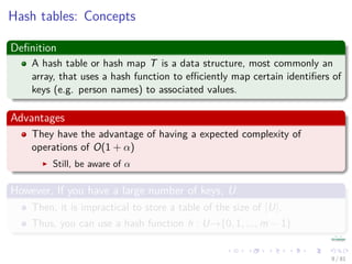
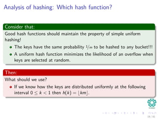
![When you have a small universe of keys, U
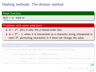
Remarks
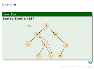
It is not necessary to map the key values.
Key values are direct addresses in the array.
Direct implementation or Direct-address tables.
Operations
1 Direct-Address-Search(T, k)
return T[k]
2 Direct-Address-Search(T, x)
T [x.key] = x
3 Direct-Address-Delete(T, x)
T [x.key] = NIL
10 / 81](https://image.slidesharecdn.com/08datastructureshashtables-150318144403-conversion-gate01/85/08-Hash-Tables-13-320.jpg)
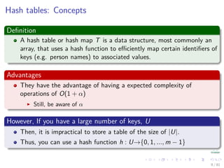
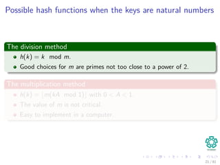
![When you have a small universe of keys, U
Remarks
It is not necessary to map the key values.
Key values are direct addresses in the array.
Direct implementation or Direct-address tables.
Operations
1 Direct-Address-Search(T, k)
return T[k]
2 Direct-Address-Search(T, x)
T [x.key] = x
3 Direct-Address-Delete(T, x)
T [x.key] = NIL
10 / 81](https://image.slidesharecdn.com/08datastructureshashtables-150318144403-conversion-gate01/85/08-Hash-Tables-14-320.jpg)

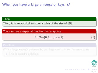


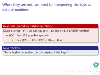

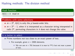


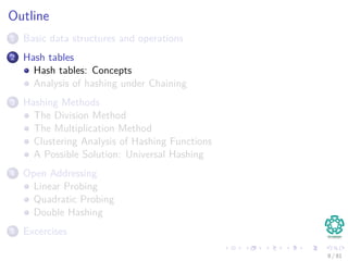
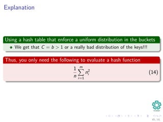
![Analysis of C: First, keys are uniformly distributed
Consider the following random variable
Consider bucket i containing ni elements, with Xij= I{element j lands in
bucket i}
Then, given
ni =
n
j=1
Xij (3)
We have that
E [Xij] =
1
m
, E X2
ij =
1
m
(4)
34 / 81](https://image.slidesharecdn.com/08datastructureshashtables-150318144403-conversion-gate01/85/08-Hash-Tables-59-320.jpg)
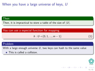
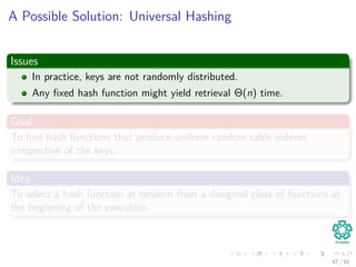
![Analysis of C: First, keys are uniformly distributed
Consider the following random variable
Consider bucket i containing ni elements, with Xij= I{element j lands in
bucket i}
Then, given
ni =
n
j=1
Xij (3)
We have that
E [Xij] =
1
m
, E X2
ij =
1
m
(4)
34 / 81](https://image.slidesharecdn.com/08datastructureshashtables-150318144403-conversion-gate01/85/08-Hash-Tables-60-320.jpg)
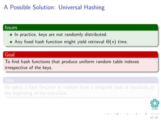
![Analysis of C: First, keys are uniformly distributed
Consider the following random variable
Consider bucket i containing ni elements, with Xij= I{element j lands in
bucket i}
Then, given
ni =
n
j=1
Xij (3)
We have that
E [Xij] =
1
m
, E X2
ij =
1
m
(4)
34 / 81](https://image.slidesharecdn.com/08datastructureshashtables-150318144403-conversion-gate01/85/08-Hash-Tables-61-320.jpg)
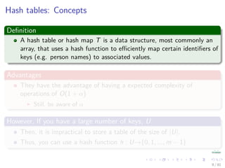
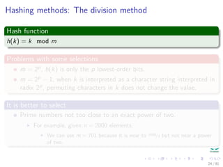
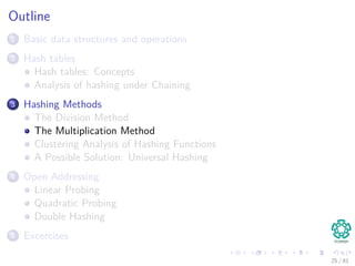
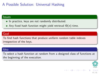
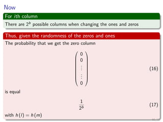
![Next
We look at the dispersion of Xij
Var [Xij] = E X2
ij − (E [Xij])2
=
1
m
−
1
m2
(5)
What about the expected number of elements at each bucket
E [ni ] = E
n
j=1
Xij
=
n
m
= α (6)
35 / 81](https://image.slidesharecdn.com/08datastructureshashtables-150318144403-conversion-gate01/85/08-Hash-Tables-62-320.jpg)
![Next
We look at the dispersion of Xij
Var [Xij] = E X2
ij − (E [Xij])2
=
1
m
−
1
m2
(5)
What about the expected number of elements at each bucket
E [ni ] = E
n
j=1
Xij
=
n
m
= α (6)
35 / 81](https://image.slidesharecdn.com/08datastructureshashtables-150318144403-conversion-gate01/85/08-Hash-Tables-63-320.jpg)
![Then, we have
Because independence of {Xij}, the scattering of ni
Var [ni ] = Var
n
j=1
Xij
=
n
j=1
Var [Xij]
= nVar [Xij]
36 / 81](https://image.slidesharecdn.com/08datastructureshashtables-150318144403-conversion-gate01/85/08-Hash-Tables-64-320.jpg)
![Then
What about the range of the possible number of elements at each
bucket?
Var [ni ] =
n
m
−
n
m2
= α −
α
m
But, we have that
E n2
i = E
n
j=1
X2
ij +
n
j=1
n
k=1,k=j
XijXik
(7)
Or
E n2
i =
n
m
+
n
j=1
n
k=1,k=j
1
m2
(8)
37 / 81](https://image.slidesharecdn.com/08datastructureshashtables-150318144403-conversion-gate01/85/08-Hash-Tables-65-320.jpg)
![Then
What about the range of the possible number of elements at each
bucket?
Var [ni ] =
n
m
−
n
m2
= α −
α
m
But, we have that
E n2
i = E
n
j=1
X2
ij +
n
j=1
n
k=1,k=j
XijXik
(7)
Or
E n2
i =
n
m
+
n
j=1
n
k=1,k=j
1
m2
(8)
37 / 81](https://image.slidesharecdn.com/08datastructureshashtables-150318144403-conversion-gate01/85/08-Hash-Tables-66-320.jpg)
![Then
What about the range of the possible number of elements at each
bucket?
Var [ni ] =
n
m
−
n
m2
= α −
α
m
But, we have that
E n2
i = E
n
j=1
X2
ij +
n
j=1
n
k=1,k=j
XijXik
(7)
Or
E n2
i =
n
m
+
n
j=1
n
k=1,k=j
1
m2
(8)
37 / 81](https://image.slidesharecdn.com/08datastructureshashtables-150318144403-conversion-gate01/85/08-Hash-Tables-67-320.jpg)
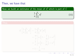
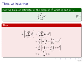
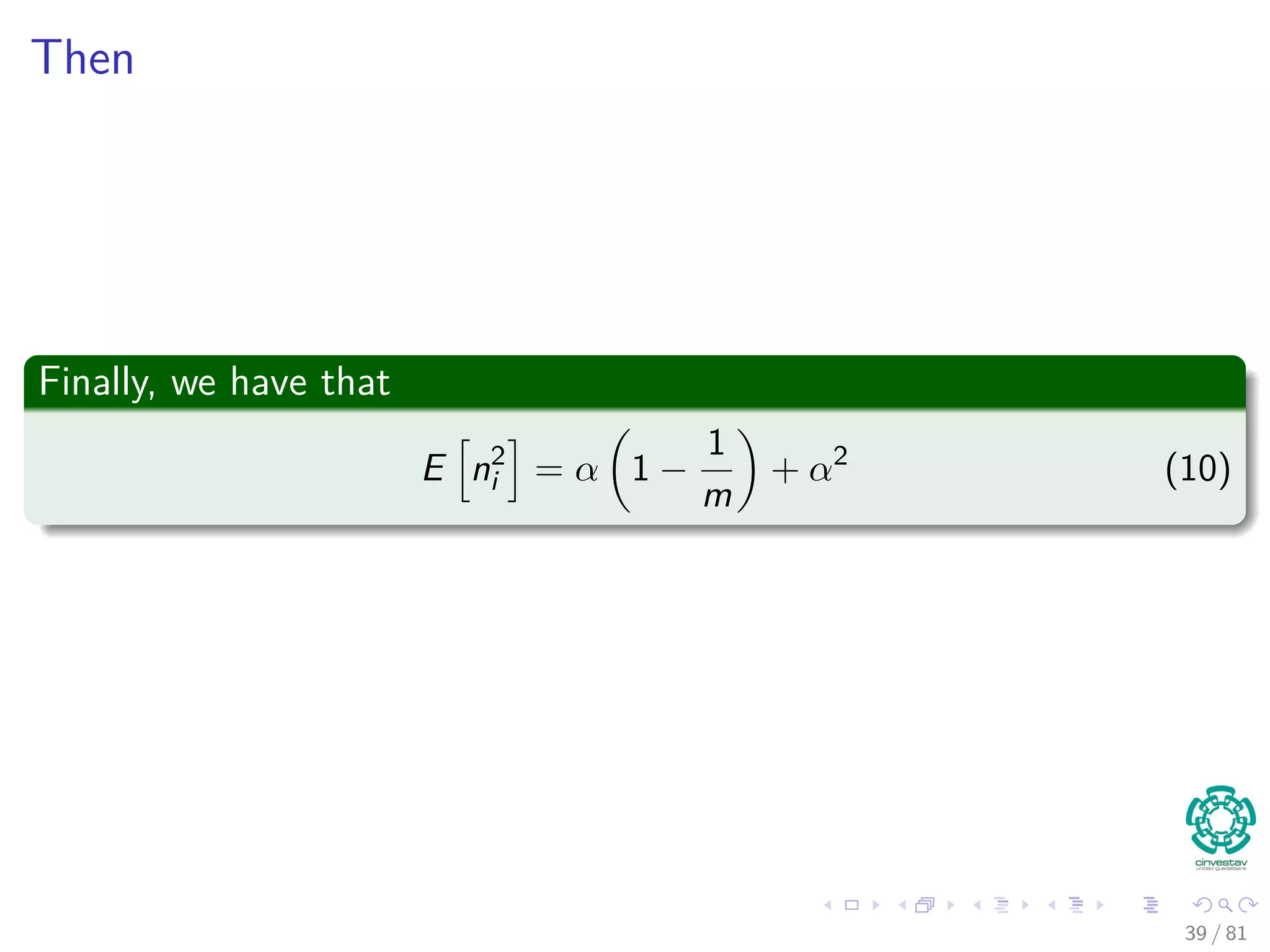
![Thus
We re-express the range on term of expected values of ni
E n2
i =
n
m
+
n (n − 1)
m2
(9)
Then
E n2
i − E [ni ]2
=
n
m
+
n (n − 1)
m2
−
n2
m2
=
n
m
−
n
m2
= α −
α
m
38 / 81](https://image.slidesharecdn.com/08datastructureshashtables-150318144403-conversion-gate01/85/08-Hash-Tables-68-320.jpg)
![Thus
We re-express the range on term of expected values of ni
E n2
i =
n
m
+
n (n − 1)
m2
(9)
Then
E n2
i − E [ni ]2
=
n
m
+
n (n − 1)
m2
−
n2
m2
=
n
m
−
n
m2
= α −
α
m
38 / 81](https://image.slidesharecdn.com/08datastructureshashtables-150318144403-conversion-gate01/85/08-Hash-Tables-69-320.jpg)
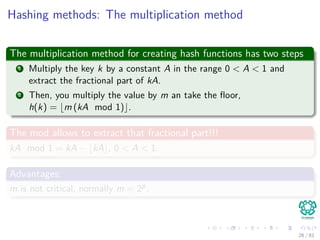
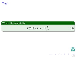
![Finally
We can plug back on C using the expected value
E [C] =
m
n − 1
E
m
i=1 n2
i
n
− 1
=
m
n − 1
1 −
1
m
+ α − 1
=
m
n − 1
n
m
−
1
m
=
m
n − 1
n − 1
m
= 1
41 / 81](https://image.slidesharecdn.com/08datastructureshashtables-150318144403-conversion-gate01/85/08-Hash-Tables-73-320.jpg)
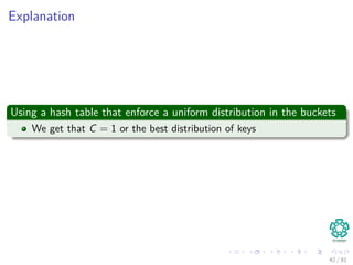
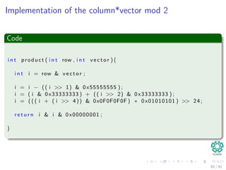
![Now, we have a really horrible hash function ≡ It hits only
one of every b buckets
Thus
E [Xij] = E X2
ij =
b
m
(12)
Thus, we have
E [ni ] = αb (13)
Then, we have
E
1
n
m
i=1
n2
i =
1
n
m
i=1
E n2
i
= αb −
b
m
+ 1
43 / 81](https://image.slidesharecdn.com/08datastructureshashtables-150318144403-conversion-gate01/85/08-Hash-Tables-75-320.jpg)
![Now, we have a really horrible hash function ≡ It hits only
one of every b buckets
Thus
E [Xij] = E X2
ij =
b
m
(12)
Thus, we have
E [ni ] = αb (13)
Then, we have
E
1
n
m
i=1
n2
i =
1
n
m
i=1
E n2
i
= αb −
b
m
+ 1
43 / 81](https://image.slidesharecdn.com/08datastructureshashtables-150318144403-conversion-gate01/85/08-Hash-Tables-76-320.jpg)
![Now, we have a really horrible hash function ≡ It hits only
one of every b buckets
Thus
E [Xij] = E X2
ij =
b
m
(12)
Thus, we have
E [ni ] = αb (13)
Then, we have
E
1
n
m
i=1
n2
i =
1
n
m
i=1
E n2
i
= αb −
b
m
+ 1
43 / 81](https://image.slidesharecdn.com/08datastructureshashtables-150318144403-conversion-gate01/85/08-Hash-Tables-77-320.jpg)
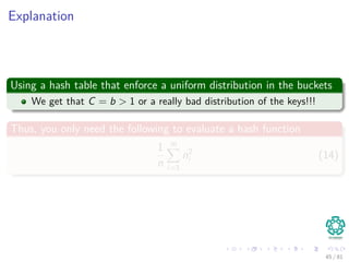
![Finally
We can plug back on C using the expected value
E [C] =
m
n − 1
E
m
i=1 n2
i
n
− 1
=
m
n − 1
αb −
b
m
+ 1 − 1
=
m
n − 1
nb
m
−
b
m
=
m
n − 1
b (n − 1)
m
= b
44 / 81](https://image.slidesharecdn.com/08datastructureshashtables-150318144403-conversion-gate01/85/08-Hash-Tables-78-320.jpg)


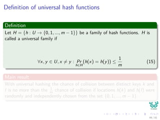
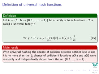
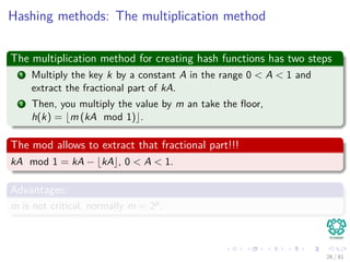
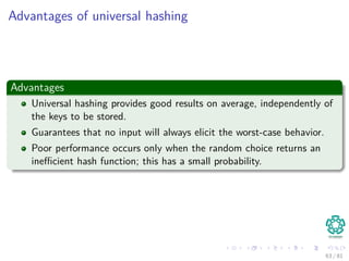
![Hashing methods: Universal hashing
Theorem 11.3
Suppose that a hash function h is chosen randomly from a universal
collection of hash functions and has been used to hash n keys into a table
T of size m, using chaining to resolve collisions. If key k is not in the
table, then the expected length E[nh(k)] of the list that key k hashes to is
at most the load factor α = n
m . If key k is in the table, then the expected
length E[nh(k)] of the list containing key k is at most 1 + α.
Corollary 11.4
Using universal hashing and collision resolution by chaining in an initially
empty table with m slots, it takes expected time Θ(n) to handle any
sequence of n INSERT, SEARCH, and DELETE operations O(m) INSERT
operations.
50 / 81](https://image.slidesharecdn.com/08datastructureshashtables-150318144403-conversion-gate01/85/08-Hash-Tables-88-320.jpg)
![Hashing methods: Universal hashing
Theorem 11.3
Suppose that a hash function h is chosen randomly from a universal
collection of hash functions and has been used to hash n keys into a table
T of size m, using chaining to resolve collisions. If key k is not in the
table, then the expected length E[nh(k)] of the list that key k hashes to is
at most the load factor α = n
m . If key k is in the table, then the expected
length E[nh(k)] of the list containing key k is at most 1 + α.
Corollary 11.4
Using universal hashing and collision resolution by chaining in an initially
empty table with m slots, it takes expected time Θ(n) to handle any
sequence of n INSERT, SEARCH, and DELETE operations O(m) INSERT
operations.
50 / 81](https://image.slidesharecdn.com/08datastructureshashtables-150318144403-conversion-gate01/85/08-Hash-Tables-89-320.jpg)
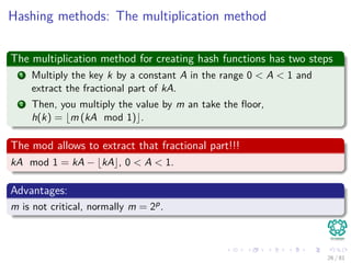
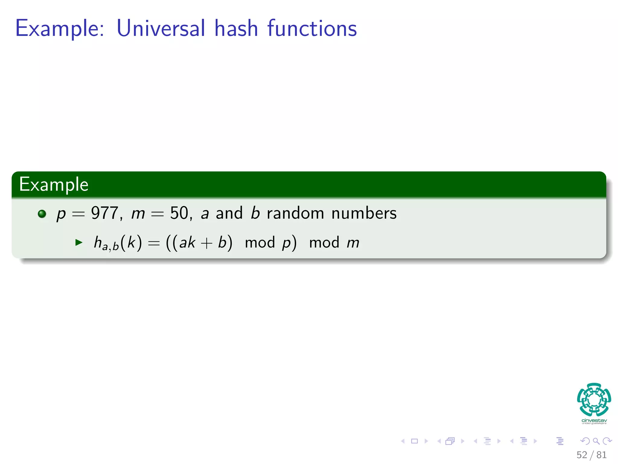
![Example of Universal Hash
Proceed as follows:
Choose a primer number p large enough so that every possible key k is in
the range [0, ..., p − 1]
Zp = {0, 1, ..., p − 1}and Z∗
p = {1, ..., p − 1}
Define the following hash function:
ha,b(k) = ((ak + b) mod p) mod m, ∀a ∈ Z∗
p and b ∈ Zp
The family of all such hash functions is:
Hp,m = {ha,b : a ∈ Z∗
p and b ∈ Zp}
Important
a and b are chosen randomly at the beginning of execution.
The class Hp,m of hash functions is universal.
51 / 81](https://image.slidesharecdn.com/08datastructureshashtables-150318144403-conversion-gate01/85/08-Hash-Tables-90-320.jpg)
![Example of Universal Hash
Proceed as follows:
Choose a primer number p large enough so that every possible key k is in
the range [0, ..., p − 1]
Zp = {0, 1, ..., p − 1}and Z∗
p = {1, ..., p − 1}
Define the following hash function:
ha,b(k) = ((ak + b) mod p) mod m, ∀a ∈ Z∗
p and b ∈ Zp
The family of all such hash functions is:
Hp,m = {ha,b : a ∈ Z∗
p and b ∈ Zp}
Important
a and b are chosen randomly at the beginning of execution.
The class Hp,m of hash functions is universal.
51 / 81](https://image.slidesharecdn.com/08datastructureshashtables-150318144403-conversion-gate01/85/08-Hash-Tables-91-320.jpg)


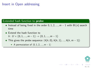
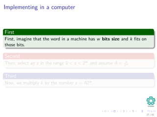
![Hashing methods in Open Addressing
HASH-INSERT(T, k)
1 i = 0
2 repeat
3 j = h (k, i)
4 if T [j] == NIL
5 T [j] = k
6 return j
7 else i = i + 1
8 until i == m
9 error “Hash Table Overflow”
66 / 81](https://image.slidesharecdn.com/08datastructureshashtables-150318144403-conversion-gate01/85/08-Hash-Tables-113-320.jpg)
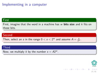
![Hashing methods in Open Addressing
HASH-SEARCH(T,k)
1 i = 0
2 repeat
3 j = h (k, i)
4 if T [j] == k
5 return j
6 i = i + 1
7 until T [j] == NIL or i == m
8 return NIL
67 / 81](https://image.slidesharecdn.com/08datastructureshashtables-150318144403-conversion-gate01/85/08-Hash-Tables-114-320.jpg)

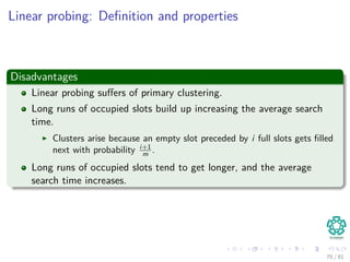
![Linear probing: Definition and properties
Hash function
Given an ordinary hash function h : 0, 1, ..., m − 1 → U for
i = 0, 1, ..., m − 1, we get the extended hash function
h(k, i) = h (k) + i mod m, (19)
Sequence of probes
Given key k, we first probe T[h (k)], then T[h (k) + 1] and so on until
T[m − 1]. Then, we wrap around T[0] to T[h (k) − 1].
Distinct probes
Because the initial probe determines the entire probe sequence, there are
m distinct probe sequences.
69 / 81](https://image.slidesharecdn.com/08datastructureshashtables-150318144403-conversion-gate01/85/08-Hash-Tables-116-320.jpg)
![Linear probing: Definition and properties
Hash function
Given an ordinary hash function h : 0, 1, ..., m − 1 → U for
i = 0, 1, ..., m − 1, we get the extended hash function
h(k, i) = h (k) + i mod m, (19)
Sequence of probes
Given key k, we first probe T[h (k)], then T[h (k) + 1] and so on until
T[m − 1]. Then, we wrap around T[0] to T[h (k) − 1].
Distinct probes
Because the initial probe determines the entire probe sequence, there are
m distinct probe sequences.
69 / 81](https://image.slidesharecdn.com/08datastructureshashtables-150318144403-conversion-gate01/85/08-Hash-Tables-117-320.jpg)
![Linear probing: Definition and properties
Hash function
Given an ordinary hash function h : 0, 1, ..., m − 1 → U for
i = 0, 1, ..., m − 1, we get the extended hash function
h(k, i) = h (k) + i mod m, (19)
Sequence of probes
Given key k, we first probe T[h (k)], then T[h (k) + 1] and so on until
T[m − 1]. Then, we wrap around T[0] to T[h (k) − 1].
Distinct probes
Because the initial probe determines the entire probe sequence, there are
m distinct probe sequences.
69 / 81](https://image.slidesharecdn.com/08datastructureshashtables-150318144403-conversion-gate01/85/08-Hash-Tables-118-320.jpg)

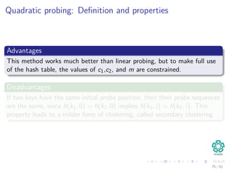
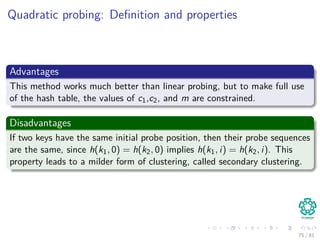
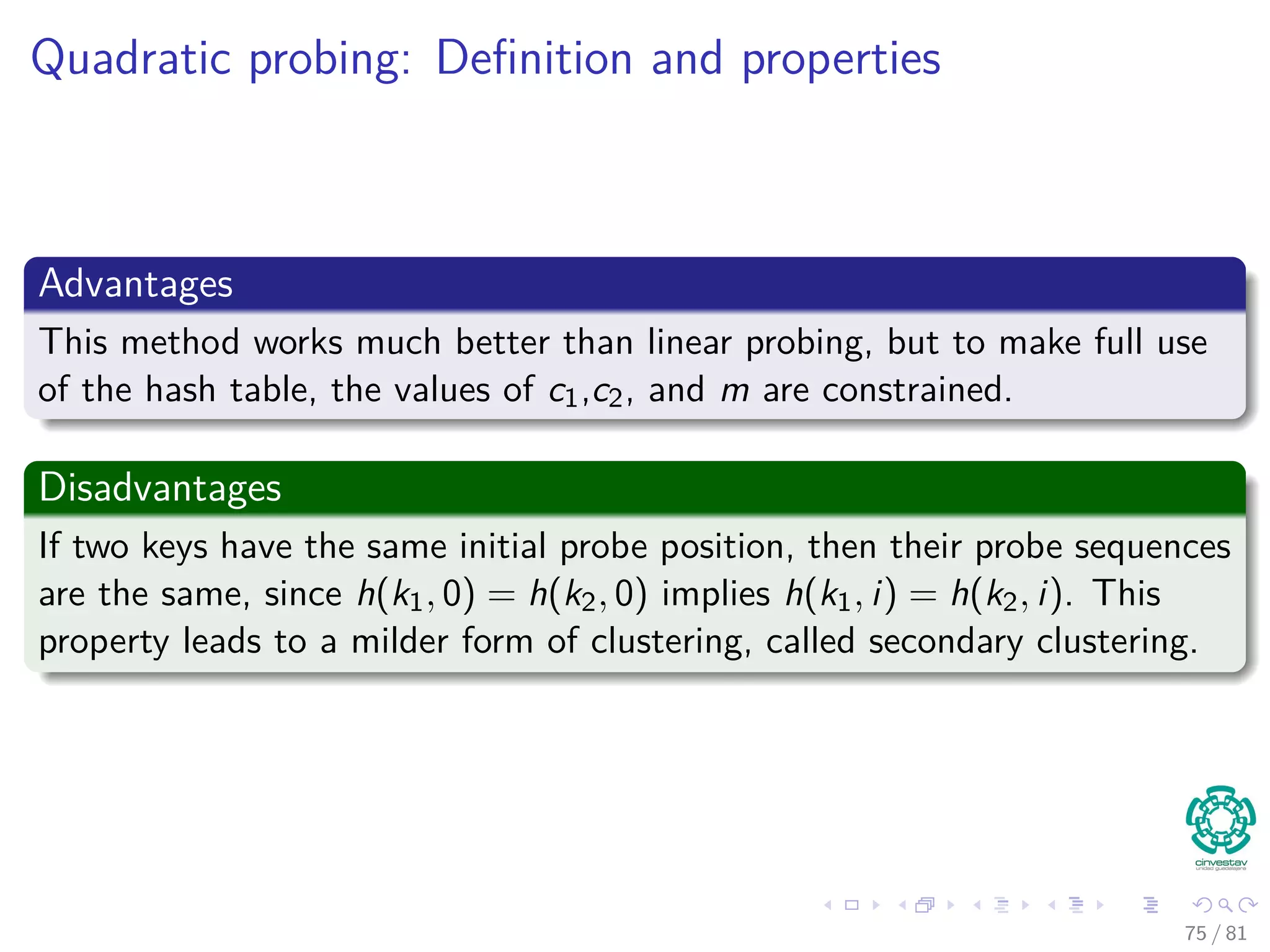
![Quadratic probing: Definition and properties
Hash function
Given an auxiliary hash function h : 0, 1, ..., m − 1 → U for
i = 0, 1, ..., m − 1, we get the extended hash function
h(k, i) = (h (k) + c1i + c2i2
) mod m, (20)
where c1, c2 are auxiliary constants
Sequence of probes
Given key k, we first probe T[h (k)], later positions probed are offset
by amounts that depend in a quadratic manner on the probe number
i.
The initial probe determines the entire sequence, and so only m
distinct probe sequences are used.
74 / 81](https://image.slidesharecdn.com/08datastructureshashtables-150318144403-conversion-gate01/85/08-Hash-Tables-125-320.jpg)
![Quadratic probing: Definition and properties
Hash function
Given an auxiliary hash function h : 0, 1, ..., m − 1 → U for
i = 0, 1, ..., m − 1, we get the extended hash function
h(k, i) = (h (k) + c1i + c2i2
) mod m, (20)
where c1, c2 are auxiliary constants
Sequence of probes
Given key k, we first probe T[h (k)], later positions probed are offset
by amounts that depend in a quadratic manner on the probe number
i.
The initial probe determines the entire sequence, and so only m
distinct probe sequences are used.
74 / 81](https://image.slidesharecdn.com/08datastructureshashtables-150318144403-conversion-gate01/85/08-Hash-Tables-126-320.jpg)
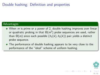
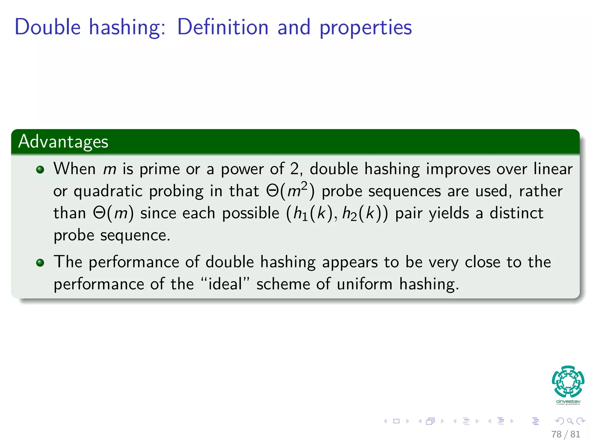
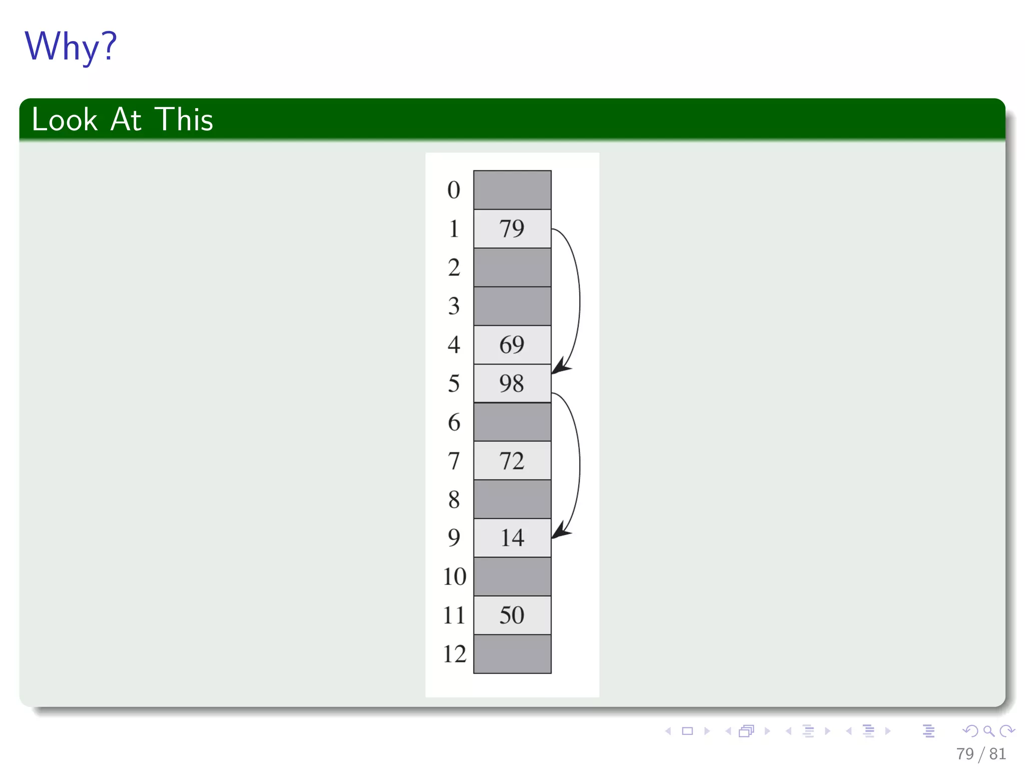
![Double hashing: Definition and properties
Hash function
Double hashing uses a hash function of the form
h(k, i) = (h1(k) + ih2(k)) mod m, (21)
where i = 0, 1, ..., m − 1 and h1, h2 are auxiliary hash functions (Normally
for a Universal family)
Sequence of probes
Given key k, we first probe T[h1(k)], successive probe positions are
offset from previous positions by the amount h2(k) mod m.
Thus, unlike the case of linear or quadratic probing, the probe
sequence here depends in two ways upon the key k, since the initial
probe position, the offset, or both, may vary.
77 / 81](https://image.slidesharecdn.com/08datastructureshashtables-150318144403-conversion-gate01/85/08-Hash-Tables-130-320.jpg)
![Double hashing: Definition and properties
Hash function
Double hashing uses a hash function of the form
h(k, i) = (h1(k) + ih2(k)) mod m, (21)
where i = 0, 1, ..., m − 1 and h1, h2 are auxiliary hash functions (Normally
for a Universal family)
Sequence of probes
Given key k, we first probe T[h1(k)], successive probe positions are
offset from previous positions by the amount h2(k) mod m.
Thus, unlike the case of linear or quadratic probing, the probe
sequence here depends in two ways upon the key k, since the initial
probe position, the offset, or both, may vary.
77 / 81](https://image.slidesharecdn.com/08datastructureshashtables-150318144403-conversion-gate01/85/08-Hash-Tables-131-320.jpg)


![When you have a small universe of keys, U
Remarks
It is not necessary to map the key values.
Key values are direct addresses in the array.
Direct implementation or Direct-address tables.
Operations
1 Direct-Address-Search(T, k)
return T[k]
2 Direct-Address-Search(T, x)
T [x.key] = x
3 Direct-Address-Delete(T, x)
T [x.key] = NIL
10 / 81](https://image.slidesharecdn.com/08datastructureshashtables-150318144403-conversion-gate01/75/08-Hash-Tables-13-2048.jpg)
![When you have a small universe of keys, U
Remarks
It is not necessary to map the key values.
Key values are direct addresses in the array.
Direct implementation or Direct-address tables.
Operations
1 Direct-Address-Search(T, k)
return T[k]
2 Direct-Address-Search(T, x)
T [x.key] = x
3 Direct-Address-Delete(T, x)
T [x.key] = NIL
10 / 81](https://image.slidesharecdn.com/08datastructureshashtables-150318144403-conversion-gate01/75/08-Hash-Tables-14-2048.jpg)


![Analysis of C: First, keys are uniformly distributed
Consider the following random variable
Consider bucket i containing ni elements, with Xij= I{element j lands in
bucket i}
Then, given
ni =
n
j=1
Xij (3)
We have that
E [Xij] =
1
m
, E X2
ij =
1
m
(4)
34 / 81](https://image.slidesharecdn.com/08datastructureshashtables-150318144403-conversion-gate01/75/08-Hash-Tables-59-2048.jpg)
![Analysis of C: First, keys are uniformly distributed
Consider the following random variable
Consider bucket i containing ni elements, with Xij= I{element j lands in
bucket i}
Then, given
ni =
n
j=1
Xij (3)
We have that
E [Xij] =
1
m
, E X2
ij =
1
m
(4)
34 / 81](https://image.slidesharecdn.com/08datastructureshashtables-150318144403-conversion-gate01/75/08-Hash-Tables-60-2048.jpg)
![Analysis of C: First, keys are uniformly distributed
Consider the following random variable
Consider bucket i containing ni elements, with Xij= I{element j lands in
bucket i}
Then, given
ni =
n
j=1
Xij (3)
We have that
E [Xij] =
1
m
, E X2
ij =
1
m
(4)
34 / 81](https://image.slidesharecdn.com/08datastructureshashtables-150318144403-conversion-gate01/75/08-Hash-Tables-61-2048.jpg)
![Next
We look at the dispersion of Xij
Var [Xij] = E X2
ij − (E [Xij])2
=
1
m
−
1
m2
(5)
What about the expected number of elements at each bucket
E [ni ] = E
n
j=1
Xij
=
n
m
= α (6)
35 / 81](https://image.slidesharecdn.com/08datastructureshashtables-150318144403-conversion-gate01/75/08-Hash-Tables-62-2048.jpg)
![Next
We look at the dispersion of Xij
Var [Xij] = E X2
ij − (E [Xij])2
=
1
m
−
1
m2
(5)
What about the expected number of elements at each bucket
E [ni ] = E
n
j=1
Xij
=
n
m
= α (6)
35 / 81](https://image.slidesharecdn.com/08datastructureshashtables-150318144403-conversion-gate01/75/08-Hash-Tables-63-2048.jpg)
![Then, we have
Because independence of {Xij}, the scattering of ni
Var [ni ] = Var
n
j=1
Xij
=
n
j=1
Var [Xij]
= nVar [Xij]
36 / 81](https://image.slidesharecdn.com/08datastructureshashtables-150318144403-conversion-gate01/75/08-Hash-Tables-64-2048.jpg)
![Then
What about the range of the possible number of elements at each
bucket?
Var [ni ] =
n
m
−
n
m2
= α −
α
m
But, we have that
E n2
i = E
n
j=1
X2
ij +
n
j=1
n
k=1,k=j
XijXik
(7)
Or
E n2
i =
n
m
+
n
j=1
n
k=1,k=j
1
m2
(8)
37 / 81](https://image.slidesharecdn.com/08datastructureshashtables-150318144403-conversion-gate01/75/08-Hash-Tables-65-2048.jpg)
![Then
What about the range of the possible number of elements at each
bucket?
Var [ni ] =
n
m
−
n
m2
= α −
α
m
But, we have that
E n2
i = E
n
j=1
X2
ij +
n
j=1
n
k=1,k=j
XijXik
(7)
Or
E n2
i =
n
m
+
n
j=1
n
k=1,k=j
1
m2
(8)
37 / 81](https://image.slidesharecdn.com/08datastructureshashtables-150318144403-conversion-gate01/75/08-Hash-Tables-66-2048.jpg)
![Then
What about the range of the possible number of elements at each
bucket?
Var [ni ] =
n
m
−
n
m2
= α −
α
m
But, we have that
E n2
i = E
n
j=1
X2
ij +
n
j=1
n
k=1,k=j
XijXik
(7)
Or
E n2
i =
n
m
+
n
j=1
n
k=1,k=j
1
m2
(8)
37 / 81](https://image.slidesharecdn.com/08datastructureshashtables-150318144403-conversion-gate01/75/08-Hash-Tables-67-2048.jpg)
![Thus
We re-express the range on term of expected values of ni
E n2
i =
n
m
+
n (n − 1)
m2
(9)
Then
E n2
i − E [ni ]2
=
n
m
+
n (n − 1)
m2
−
n2
m2
=
n
m
−
n
m2
= α −
α
m
38 / 81](https://image.slidesharecdn.com/08datastructureshashtables-150318144403-conversion-gate01/75/08-Hash-Tables-68-2048.jpg)
![Thus
We re-express the range on term of expected values of ni
E n2
i =
n
m
+
n (n − 1)
m2
(9)
Then
E n2
i − E [ni ]2
=
n
m
+
n (n − 1)
m2
−
n2
m2
=
n
m
−
n
m2
= α −
α
m
38 / 81](https://image.slidesharecdn.com/08datastructureshashtables-150318144403-conversion-gate01/75/08-Hash-Tables-69-2048.jpg)
![Finally
We can plug back on C using the expected value
E [C] =
m
n − 1
E
m
i=1 n2
i
n
− 1
=
m
n − 1
1 −
1
m
+ α − 1
=
m
n − 1
n
m
−
1
m
=
m
n − 1
n − 1
m
= 1
41 / 81](https://image.slidesharecdn.com/08datastructureshashtables-150318144403-conversion-gate01/75/08-Hash-Tables-73-2048.jpg)

![Now, we have a really horrible hash function ≡ It hits only
one of every b buckets
Thus
E [Xij] = E X2
ij =
b
m
(12)
Thus, we have
E [ni ] = αb (13)
Then, we have
E
1
n
m
i=1
n2
i =
1
n
m
i=1
E n2
i
= αb −
b
m
+ 1
43 / 81](https://image.slidesharecdn.com/08datastructureshashtables-150318144403-conversion-gate01/75/08-Hash-Tables-75-2048.jpg)
![Now, we have a really horrible hash function ≡ It hits only
one of every b buckets
Thus
E [Xij] = E X2
ij =
b
m
(12)
Thus, we have
E [ni ] = αb (13)
Then, we have
E
1
n
m
i=1
n2
i =
1
n
m
i=1
E n2
i
= αb −
b
m
+ 1
43 / 81](https://image.slidesharecdn.com/08datastructureshashtables-150318144403-conversion-gate01/75/08-Hash-Tables-76-2048.jpg)
![Now, we have a really horrible hash function ≡ It hits only
one of every b buckets
Thus
E [Xij] = E X2
ij =
b
m
(12)
Thus, we have
E [ni ] = αb (13)
Then, we have
E
1
n
m
i=1
n2
i =
1
n
m
i=1
E n2
i
= αb −
b
m
+ 1
43 / 81](https://image.slidesharecdn.com/08datastructureshashtables-150318144403-conversion-gate01/75/08-Hash-Tables-77-2048.jpg)
![Finally
We can plug back on C using the expected value
E [C] =
m
n − 1
E
m
i=1 n2
i
n
− 1
=
m
n − 1
αb −
b
m
+ 1 − 1
=
m
n − 1
nb
m
−
b
m
=
m
n − 1
b (n − 1)
m
= b
44 / 81](https://image.slidesharecdn.com/08datastructureshashtables-150318144403-conversion-gate01/75/08-Hash-Tables-78-2048.jpg)

![Hashing methods: Universal hashing
Theorem 11.3
Suppose that a hash function h is chosen randomly from a universal
collection of hash functions and has been used to hash n keys into a table
T of size m, using chaining to resolve collisions. If key k is not in the
table, then the expected length E[nh(k)] of the list that key k hashes to is
at most the load factor α = n
m . If key k is in the table, then the expected
length E[nh(k)] of the list containing key k is at most 1 + α.
Corollary 11.4
Using universal hashing and collision resolution by chaining in an initially
empty table with m slots, it takes expected time Θ(n) to handle any
sequence of n INSERT, SEARCH, and DELETE operations O(m) INSERT
operations.
50 / 81](https://image.slidesharecdn.com/08datastructureshashtables-150318144403-conversion-gate01/75/08-Hash-Tables-88-2048.jpg)
![Hashing methods: Universal hashing
Theorem 11.3
Suppose that a hash function h is chosen randomly from a universal
collection of hash functions and has been used to hash n keys into a table
T of size m, using chaining to resolve collisions. If key k is not in the
table, then the expected length E[nh(k)] of the list that key k hashes to is
at most the load factor α = n
m . If key k is in the table, then the expected
length E[nh(k)] of the list containing key k is at most 1 + α.
Corollary 11.4
Using universal hashing and collision resolution by chaining in an initially
empty table with m slots, it takes expected time Θ(n) to handle any
sequence of n INSERT, SEARCH, and DELETE operations O(m) INSERT
operations.
50 / 81](https://image.slidesharecdn.com/08datastructureshashtables-150318144403-conversion-gate01/75/08-Hash-Tables-89-2048.jpg)
![Example of Universal Hash
Proceed as follows:
Choose a primer number p large enough so that every possible key k is in
the range [0, ..., p − 1]
Zp = {0, 1, ..., p − 1}and Z∗
p = {1, ..., p − 1}
Define the following hash function:
ha,b(k) = ((ak + b) mod p) mod m, ∀a ∈ Z∗
p and b ∈ Zp
The family of all such hash functions is:
Hp,m = {ha,b : a ∈ Z∗
p and b ∈ Zp}
Important
a and b are chosen randomly at the beginning of execution.
The class Hp,m of hash functions is universal.
51 / 81](https://image.slidesharecdn.com/08datastructureshashtables-150318144403-conversion-gate01/75/08-Hash-Tables-90-2048.jpg)
![Example of Universal Hash
Proceed as follows:
Choose a primer number p large enough so that every possible key k is in
the range [0, ..., p − 1]
Zp = {0, 1, ..., p − 1}and Z∗
p = {1, ..., p − 1}
Define the following hash function:
ha,b(k) = ((ak + b) mod p) mod m, ∀a ∈ Z∗
p and b ∈ Zp
The family of all such hash functions is:
Hp,m = {ha,b : a ∈ Z∗
p and b ∈ Zp}
Important
a and b are chosen randomly at the beginning of execution.
The class Hp,m of hash functions is universal.
51 / 81](https://image.slidesharecdn.com/08datastructureshashtables-150318144403-conversion-gate01/75/08-Hash-Tables-91-2048.jpg)


![Hashing methods in Open Addressing
HASH-INSERT(T, k)
1 i = 0
2 repeat
3 j = h (k, i)
4 if T [j] == NIL
5 T [j] = k
6 return j
7 else i = i + 1
8 until i == m
9 error “Hash Table Overflow”
66 / 81](https://image.slidesharecdn.com/08datastructureshashtables-150318144403-conversion-gate01/75/08-Hash-Tables-113-2048.jpg)
![Hashing methods in Open Addressing
HASH-SEARCH(T,k)
1 i = 0
2 repeat
3 j = h (k, i)
4 if T [j] == k
5 return j
6 i = i + 1
7 until T [j] == NIL or i == m
8 return NIL
67 / 81](https://image.slidesharecdn.com/08datastructureshashtables-150318144403-conversion-gate01/75/08-Hash-Tables-114-2048.jpg)
![Linear probing: Definition and properties
Hash function
Given an ordinary hash function h : 0, 1, ..., m − 1 → U for
i = 0, 1, ..., m − 1, we get the extended hash function
h(k, i) = h (k) + i mod m, (19)
Sequence of probes
Given key k, we first probe T[h (k)], then T[h (k) + 1] and so on until
T[m − 1]. Then, we wrap around T[0] to T[h (k) − 1].
Distinct probes
Because the initial probe determines the entire probe sequence, there are
m distinct probe sequences.
69 / 81](https://image.slidesharecdn.com/08datastructureshashtables-150318144403-conversion-gate01/75/08-Hash-Tables-116-2048.jpg)
![Linear probing: Definition and properties
Hash function
Given an ordinary hash function h : 0, 1, ..., m − 1 → U for
i = 0, 1, ..., m − 1, we get the extended hash function
h(k, i) = h (k) + i mod m, (19)
Sequence of probes
Given key k, we first probe T[h (k)], then T[h (k) + 1] and so on until
T[m − 1]. Then, we wrap around T[0] to T[h (k) − 1].
Distinct probes
Because the initial probe determines the entire probe sequence, there are
m distinct probe sequences.
69 / 81](https://image.slidesharecdn.com/08datastructureshashtables-150318144403-conversion-gate01/75/08-Hash-Tables-117-2048.jpg)
![Linear probing: Definition and properties
Hash function
Given an ordinary hash function h : 0, 1, ..., m − 1 → U for
i = 0, 1, ..., m − 1, we get the extended hash function
h(k, i) = h (k) + i mod m, (19)
Sequence of probes
Given key k, we first probe T[h (k)], then T[h (k) + 1] and so on until
T[m − 1]. Then, we wrap around T[0] to T[h (k) − 1].
Distinct probes
Because the initial probe determines the entire probe sequence, there are
m distinct probe sequences.
69 / 81](https://image.slidesharecdn.com/08datastructureshashtables-150318144403-conversion-gate01/75/08-Hash-Tables-118-2048.jpg)
![Quadratic probing: Definition and properties
Hash function
Given an auxiliary hash function h : 0, 1, ..., m − 1 → U for
i = 0, 1, ..., m − 1, we get the extended hash function
h(k, i) = (h (k) + c1i + c2i2
) mod m, (20)
where c1, c2 are auxiliary constants
Sequence of probes
Given key k, we first probe T[h (k)], later positions probed are offset
by amounts that depend in a quadratic manner on the probe number
i.
The initial probe determines the entire sequence, and so only m
distinct probe sequences are used.
74 / 81](https://image.slidesharecdn.com/08datastructureshashtables-150318144403-conversion-gate01/75/08-Hash-Tables-125-2048.jpg)
![Quadratic probing: Definition and properties
Hash function
Given an auxiliary hash function h : 0, 1, ..., m − 1 → U for
i = 0, 1, ..., m − 1, we get the extended hash function
h(k, i) = (h (k) + c1i + c2i2
) mod m, (20)
where c1, c2 are auxiliary constants
Sequence of probes
Given key k, we first probe T[h (k)], later positions probed are offset
by amounts that depend in a quadratic manner on the probe number
i.
The initial probe determines the entire sequence, and so only m
distinct probe sequences are used.
74 / 81](https://image.slidesharecdn.com/08datastructureshashtables-150318144403-conversion-gate01/75/08-Hash-Tables-126-2048.jpg)

![Double hashing: Definition and properties
Hash function
Double hashing uses a hash function of the form
h(k, i) = (h1(k) + ih2(k)) mod m, (21)
where i = 0, 1, ..., m − 1 and h1, h2 are auxiliary hash functions (Normally
for a Universal family)
Sequence of probes
Given key k, we first probe T[h1(k)], successive probe positions are
offset from previous positions by the amount h2(k) mod m.
Thus, unlike the case of linear or quadratic probing, the probe
sequence here depends in two ways upon the key k, since the initial
probe position, the offset, or both, may vary.
77 / 81](https://image.slidesharecdn.com/08datastructureshashtables-150318144403-conversion-gate01/75/08-Hash-Tables-130-2048.jpg)
![Double hashing: Definition and properties
Hash function
Double hashing uses a hash function of the form
h(k, i) = (h1(k) + ih2(k)) mod m, (21)
where i = 0, 1, ..., m − 1 and h1, h2 are auxiliary hash functions (Normally
for a Universal family)
Sequence of probes
Given key k, we first probe T[h1(k)], successive probe positions are
offset from previous positions by the amount h2(k) mod m.
Thus, unlike the case of linear or quadratic probing, the probe
sequence here depends in two ways upon the key k, since the initial
probe position, the offset, or both, may vary.
77 / 81](https://image.slidesharecdn.com/08datastructureshashtables-150318144403-conversion-gate01/75/08-Hash-Tables-131-2048.jpg)


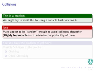
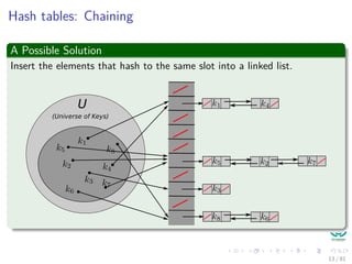
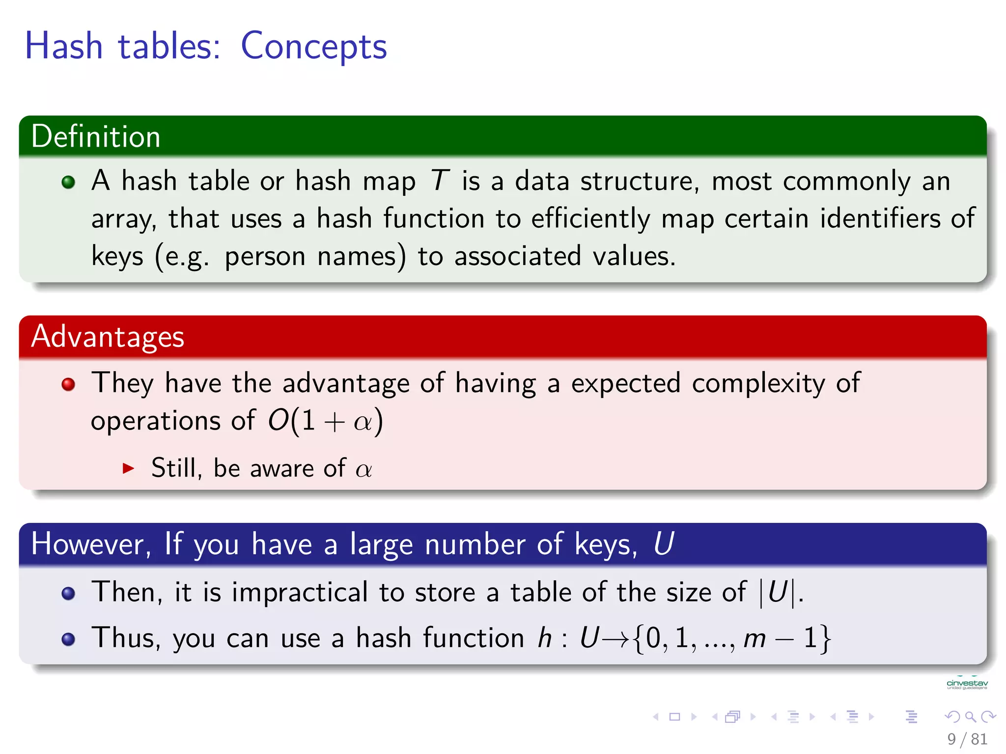
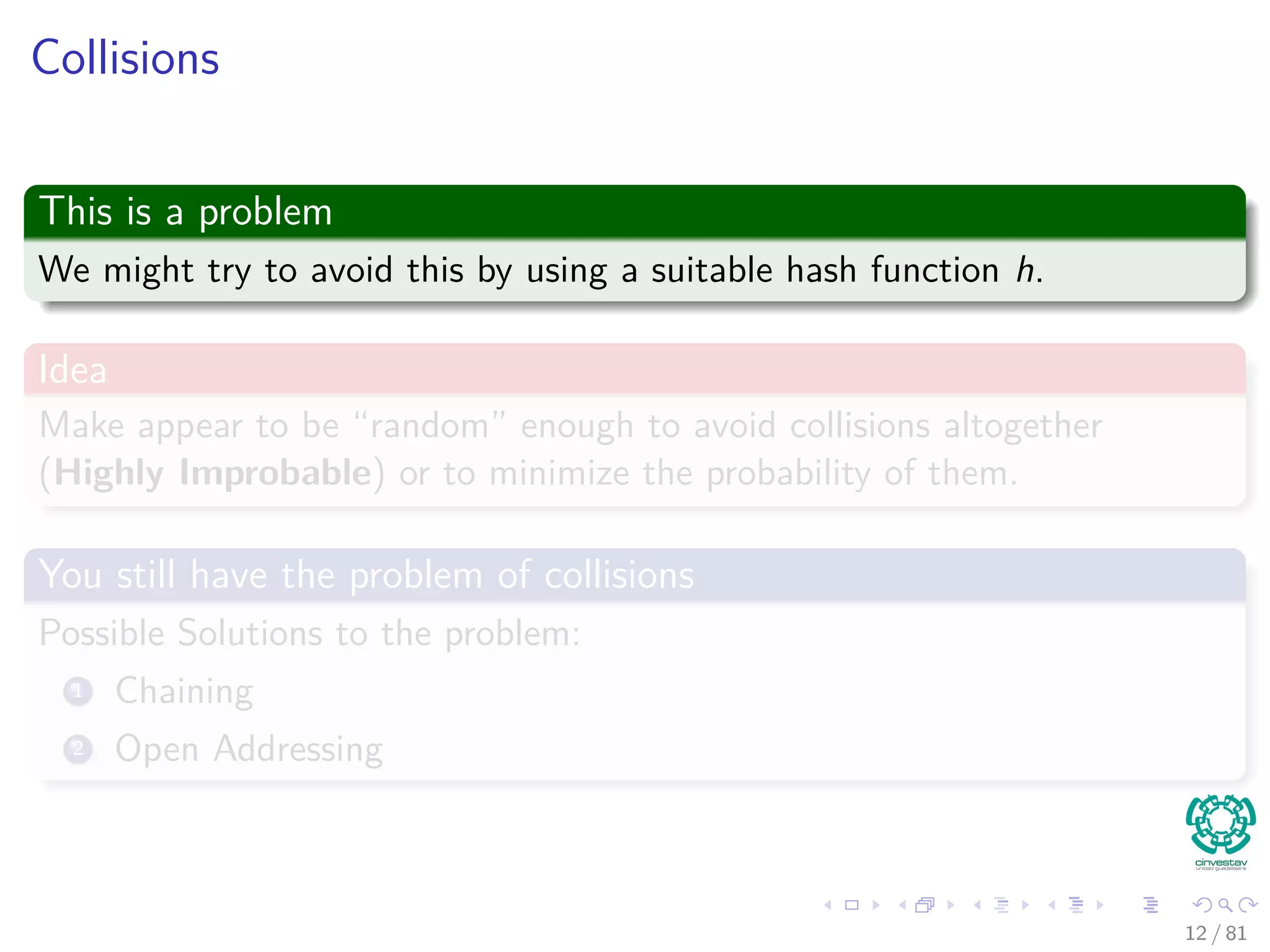
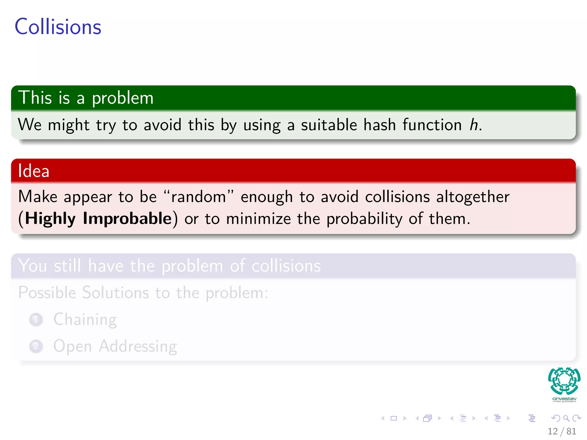
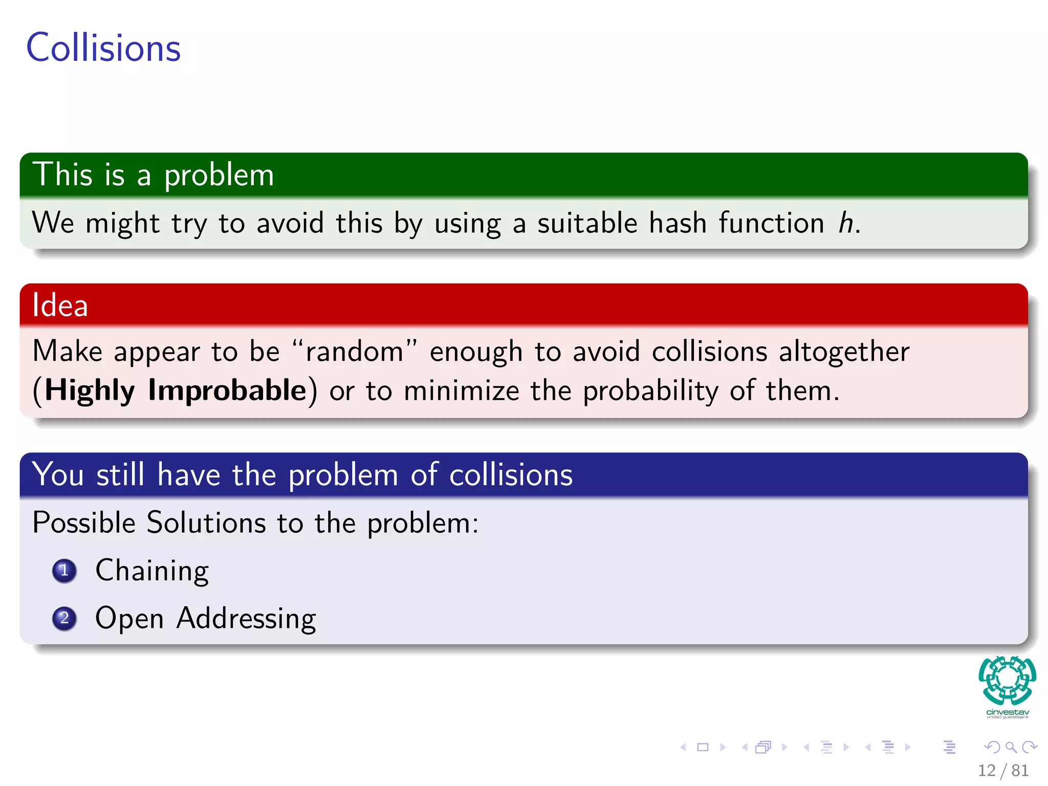
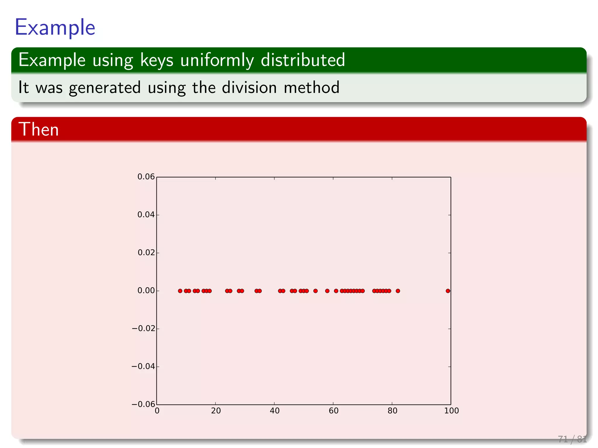
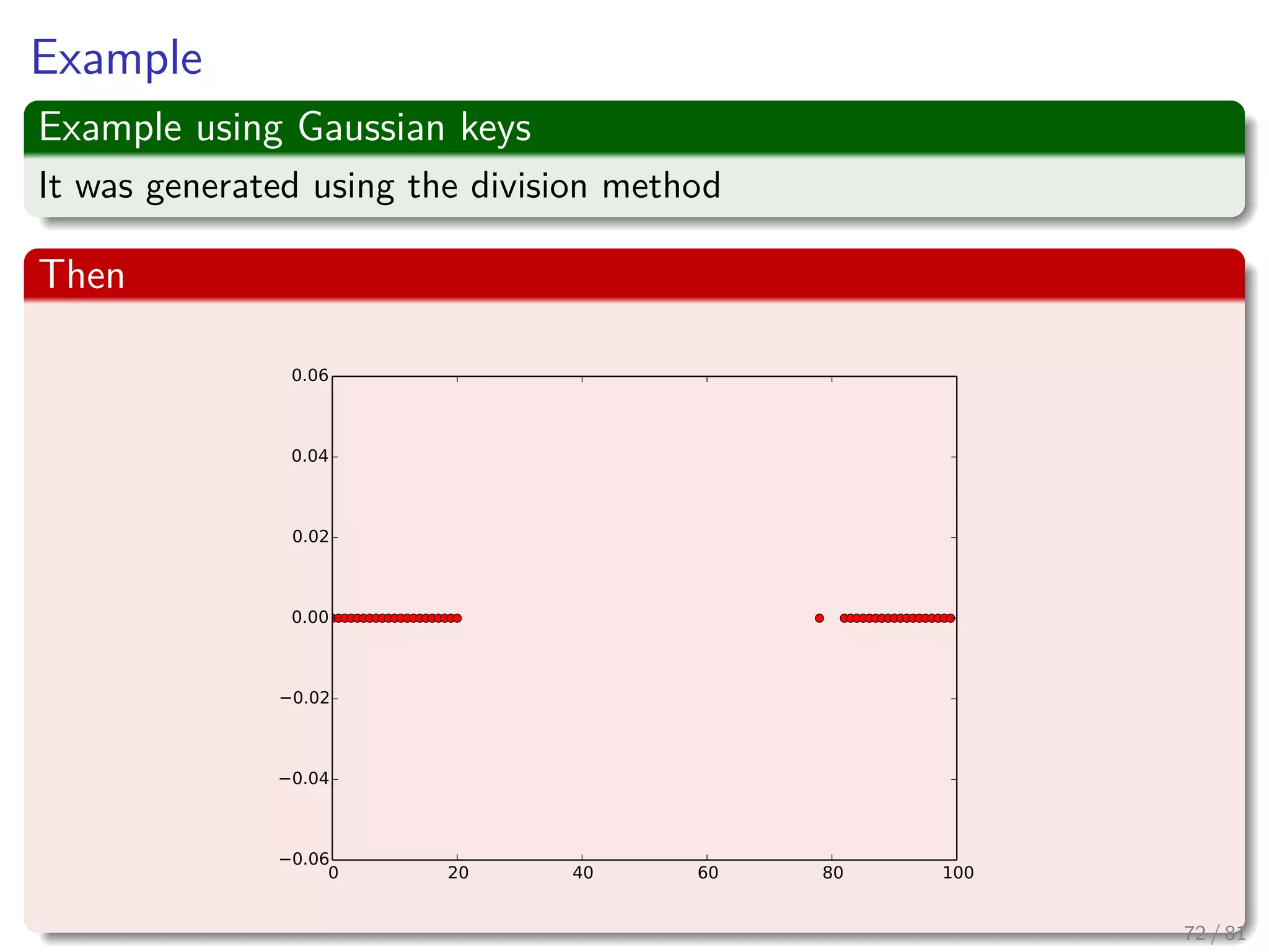
The document provides a comprehensive analysis of hash tables, covering basic data structures, hash table concepts, hashing methods, and their performance. It discusses challenges like collisions and strategies such as chaining and open addressing to resolve them. The text also emphasizes the importance of selecting effective hash functions to ensure efficient data storage and retrieval.


