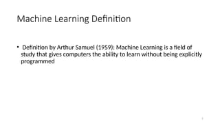
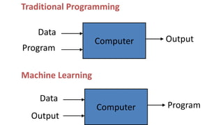
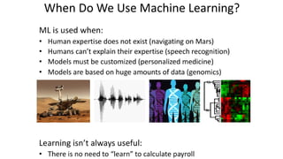
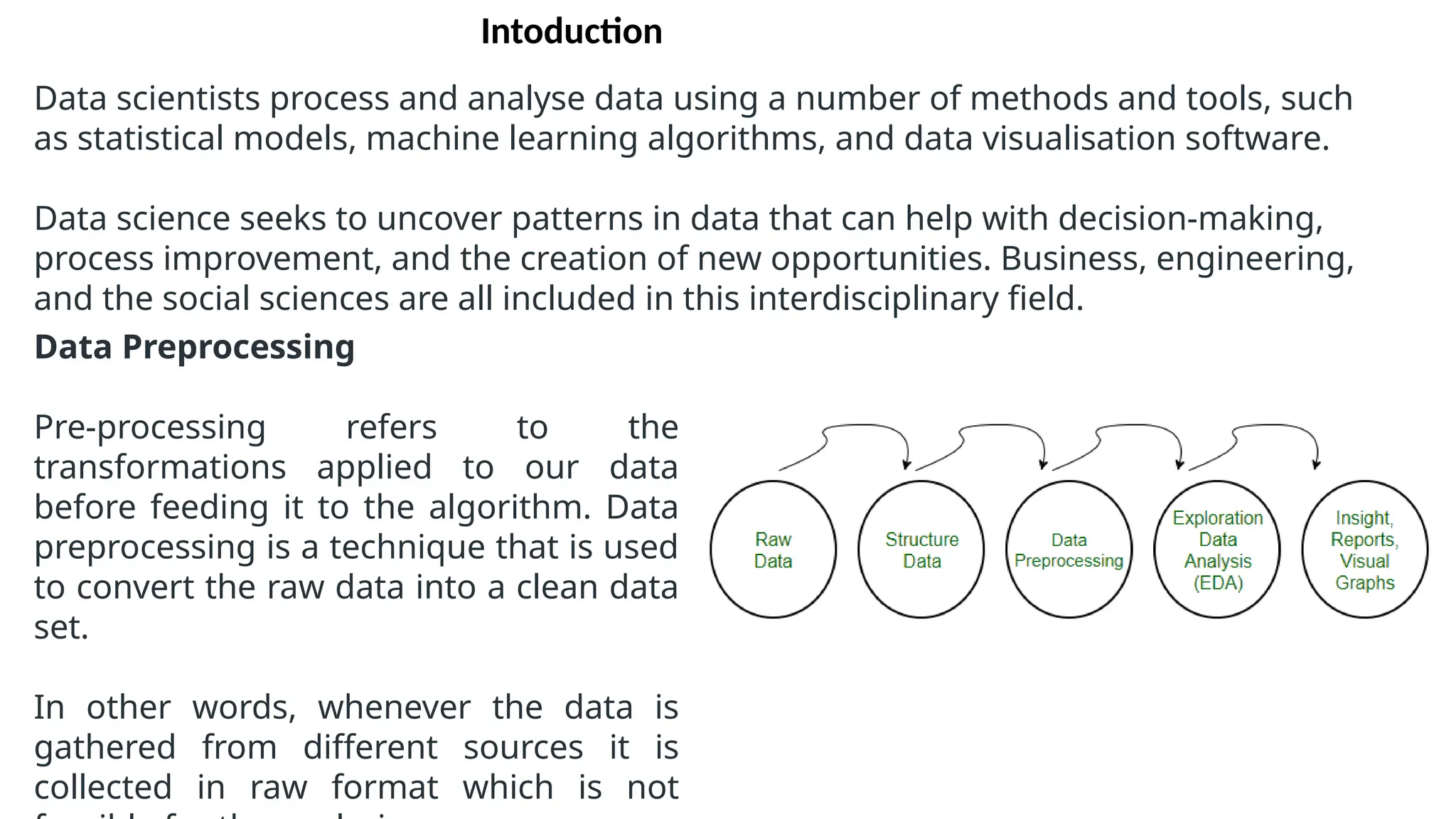
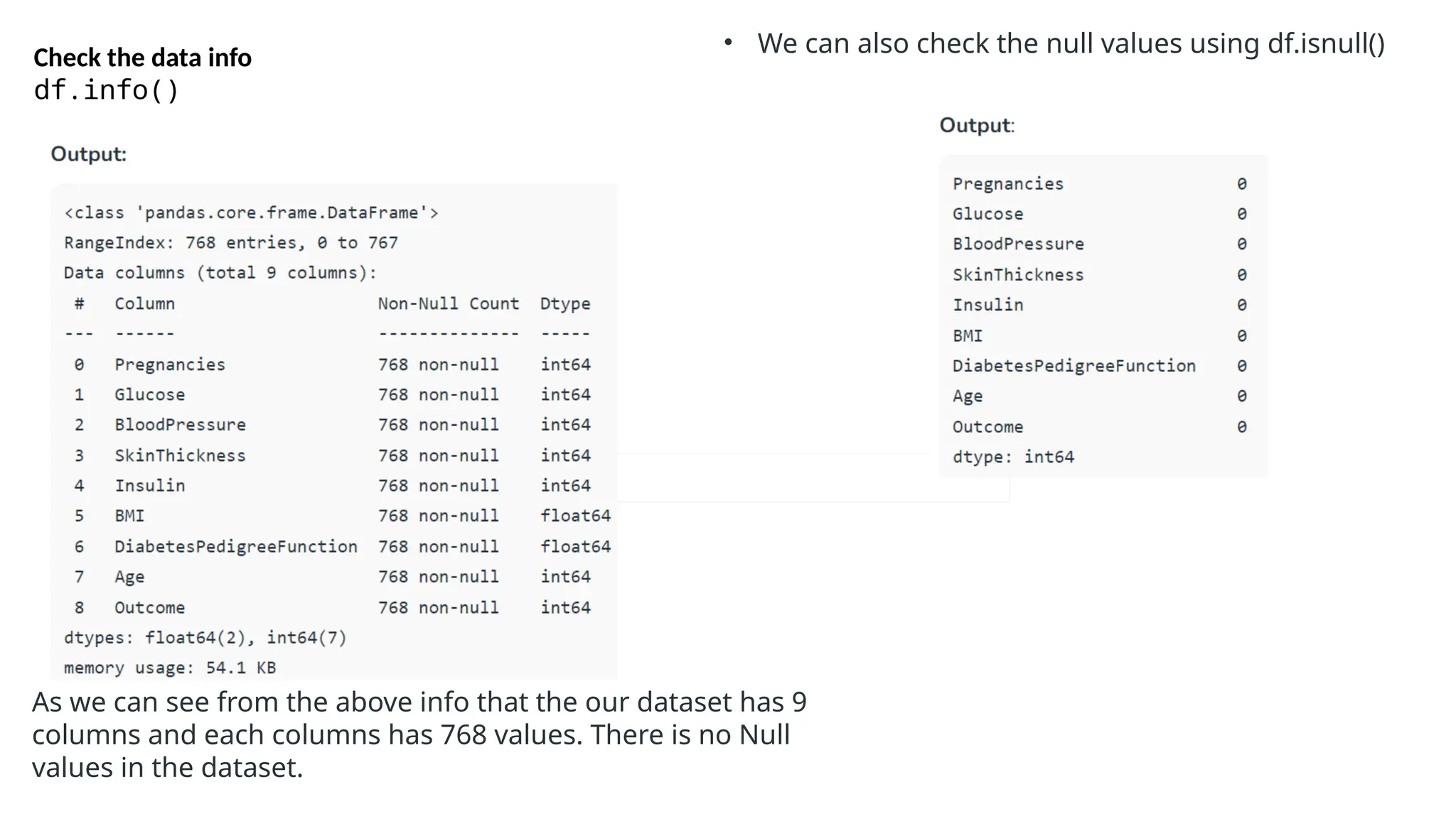
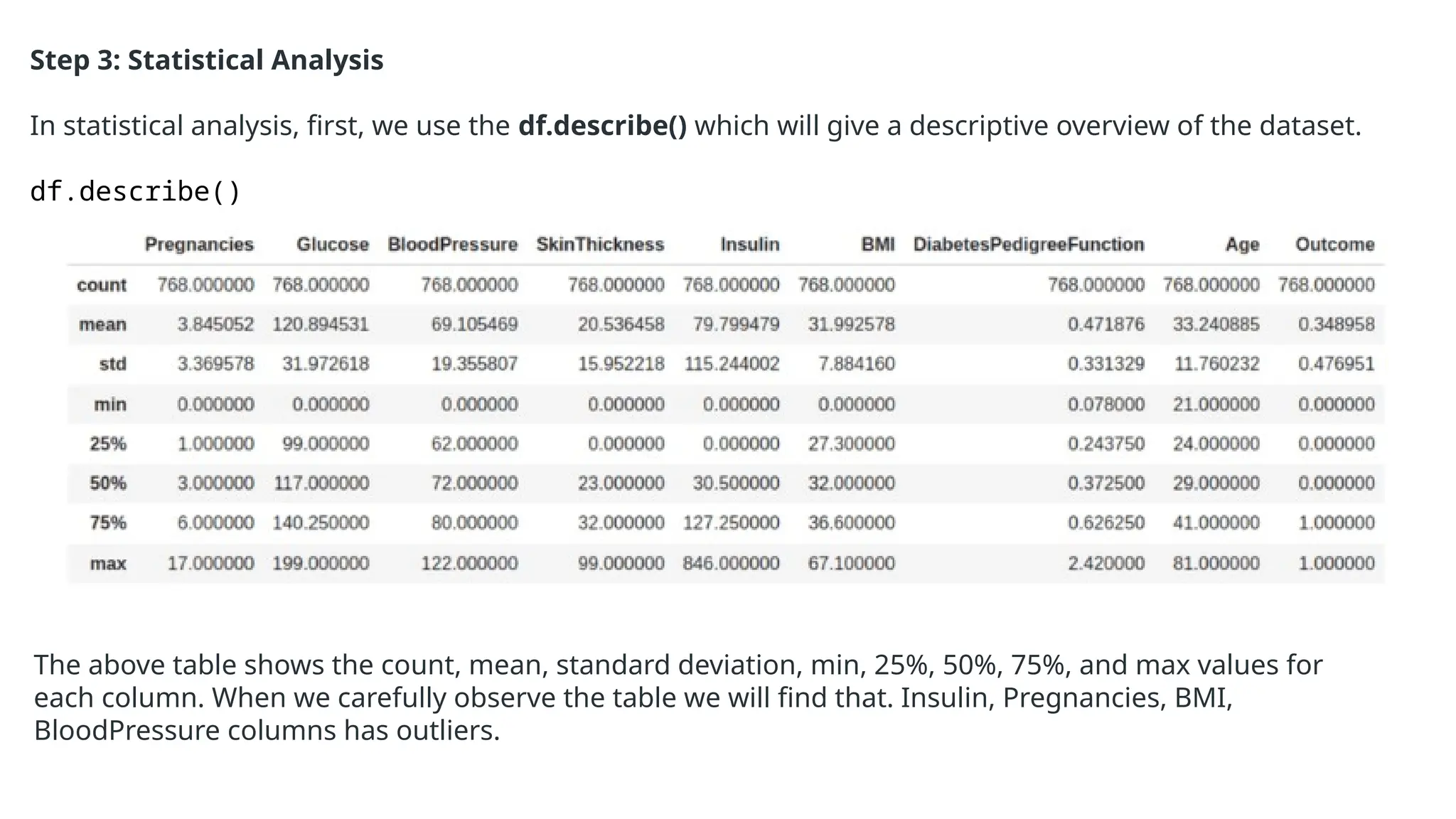
The document provides an overview of machine learning and data preprocessing techniques essential for preparing data before applying machine learning models. It details steps involved in data preprocessing such as importing libraries, loading datasets, performing statistical analysis, checking for outliers, and normalizing or standardizing data. Key concepts include the significance of data formatting for model execution and the use of specific algorithms to manage null values and format datasets appropriately.

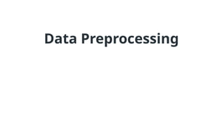

![Let’s plot the boxplot for each column for easy understanding.
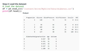
Step 4: Check the outliers:
# Box Plots
fig, axs = plt.subplots(9,1,dpi=95, figsize=(7,17))
i = 0
for col in df.columns:
axs[i].boxplot(df[col], vert=False)
axs[i].set_ylabel(col)
i+=1
plt.show()](https://image.slidesharecdn.com/introductiontomldatapreprocessing-241006023029-d230baeb/85/Introduction-to-ML_Data-Preprocessing-pptx-17-320.jpg)
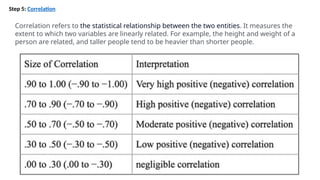
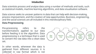
![Step 5: Correlation
#correlation
corr = df.corr()
plt.figure(dpi=130)
sns.heatmap(df.corr(), annot=True,
fmt= '.2f')
plt.show()
corr['Outcome'].sort_values(ascend
ing = Falase
We can also camapare by single columns in
descending order](https://image.slidesharecdn.com/introductiontomldatapreprocessing-241006023029-d230baeb/85/Introduction-to-ML_Data-Preprocessing-pptx-19-320.jpg)
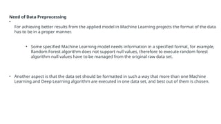
![Step 6: Separate independent features and Target Variables
# separate array into input and output components
X = df.drop(columns =['Outcome'])
Y = df.Outcome
Step 7: Normalization or Standardization
Normalization
• MinMaxScaler scales the data so that each feature is in the range [0, 1].
• It works well when the features have different scales and the algorithm being used is sensitive to the
scale of the features, such as k-nearest neighbors or neural networks.
• Rescale your data using scikit-learn using the MinMaxScaler.
Standardization
• Standardization is a useful technique to transform attributes with a Gaussian distribution and
differing means and standard deviations to a standard Gaussian distribution with a mean of 0 and a
standard deviation of 1.
• We can standardize data using scikit-learn with the StandardScaler class.
• It works well when the features have a normal distribution or when the algorithm being used is not
sensitive to the scale of the features](https://image.slidesharecdn.com/introductiontomldatapreprocessing-241006023029-d230baeb/85/Introduction-to-ML_Data-Preprocessing-pptx-20-320.jpg)


![Let’s plot the boxplot for each column for easy understanding.
Step 4: Check the outliers:
# Box Plots
fig, axs = plt.subplots(9,1,dpi=95, figsize=(7,17))
i = 0
for col in df.columns:
axs[i].boxplot(df[col], vert=False)
axs[i].set_ylabel(col)
i+=1
plt.show()](https://image.slidesharecdn.com/introductiontomldatapreprocessing-241006023029-d230baeb/75/Introduction-to-ML_Data-Preprocessing-pptx-17-2048.jpg)

![Step 5: Correlation
#correlation
corr = df.corr()
plt.figure(dpi=130)
sns.heatmap(df.corr(), annot=True,
fmt= '.2f')
plt.show()
corr['Outcome'].sort_values(ascend
ing = Falase
We can also camapare by single columns in
descending order](https://image.slidesharecdn.com/introductiontomldatapreprocessing-241006023029-d230baeb/75/Introduction-to-ML_Data-Preprocessing-pptx-19-2048.jpg)
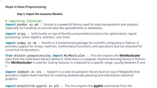
![Step 6: Separate independent features and Target Variables
# separate array into input and output components
X = df.drop(columns =['Outcome'])
Y = df.Outcome
Step 7: Normalization or Standardization
Normalization
• MinMaxScaler scales the data so that each feature is in the range [0, 1].
• It works well when the features have different scales and the algorithm being used is sensitive to the
scale of the features, such as k-nearest neighbors or neural networks.
• Rescale your data using scikit-learn using the MinMaxScaler.
Standardization
• Standardization is a useful technique to transform attributes with a Gaussian distribution and
differing means and standard deviations to a standard Gaussian distribution with a mean of 0 and a
standard deviation of 1.
• We can standardize data using scikit-learn with the StandardScaler class.
• It works well when the features have a normal distribution or when the algorithm being used is not
sensitive to the scale of the features](https://image.slidesharecdn.com/introductiontomldatapreprocessing-241006023029-d230baeb/75/Introduction-to-ML_Data-Preprocessing-pptx-20-2048.jpg)