Downloaded 334 times
![5
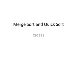
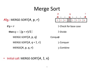
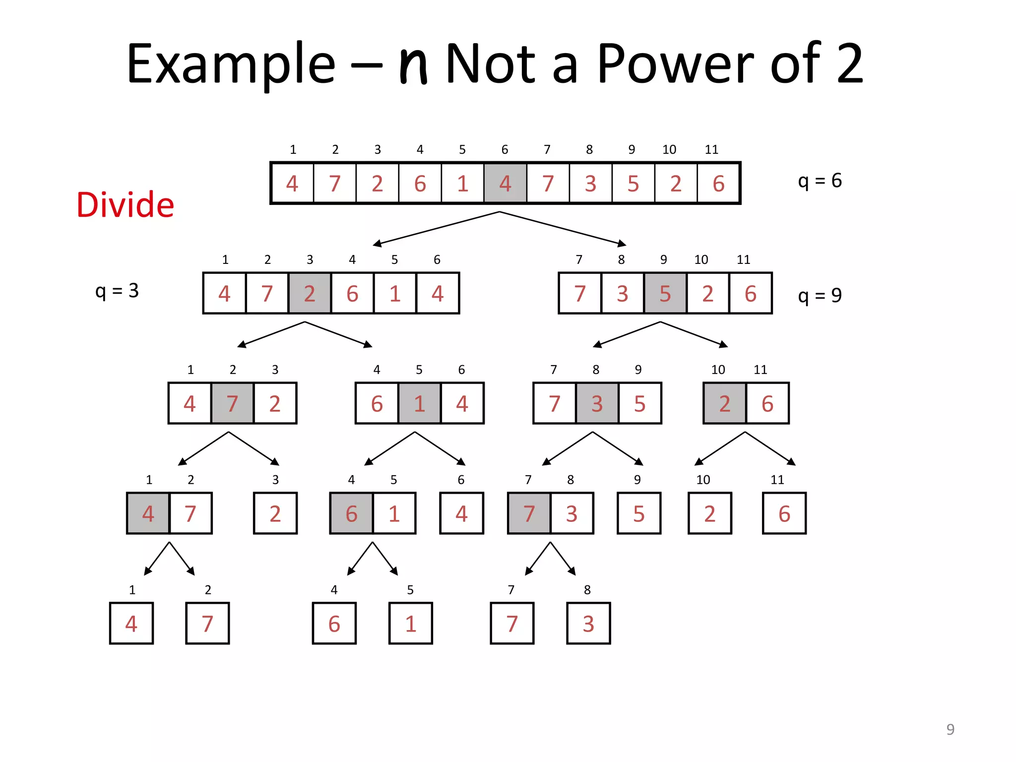
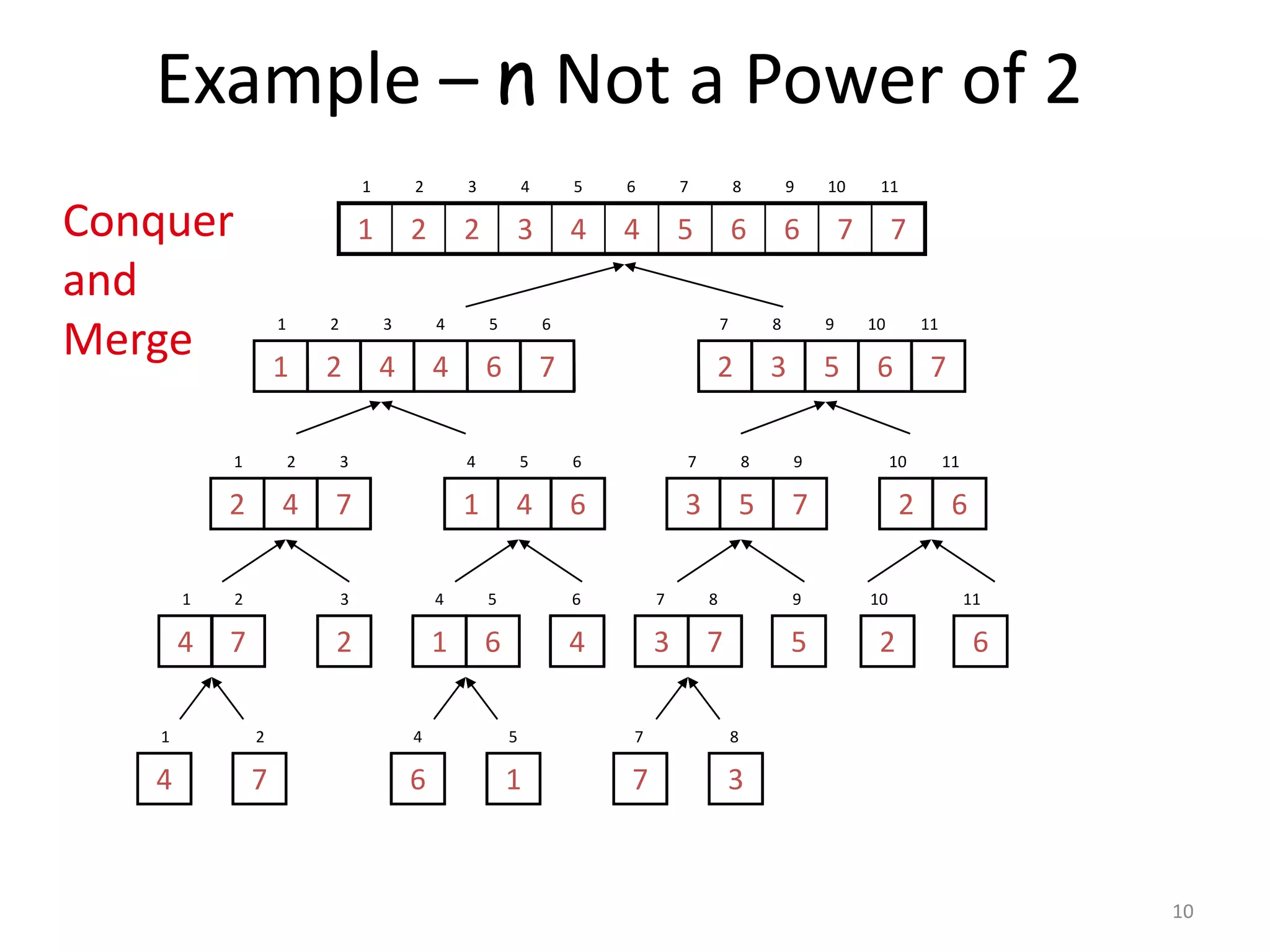
Merge Sort Approach
• To sort an array A[p . . r]:
• Divide
– Divide the n-element sequence to be sorted into two
subsequences of n/2 elements each
• Conquer
– Sort the subsequences recursively using merge sort
– When the size of the sequences is 1 there is nothing
more to do
• Combine
– Merge the two sorted subsequences](https://image.slidesharecdn.com/mergesortandquicksort-140701050833-phpapp01/85/Merge-sort-and-quick-sort-5-320.jpg)
![11
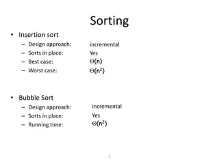
Merge - Pseudocode
Alg.: MERGE(A, p, q, r)
1. Compute n1 and n2
2. Copy the first n1 elements into L[1
. . n1 + 1] and the next n2 elements into R[1 . . n2 + 1]
3. L[n1 + 1] ← ; R[n2 + 1] ←
4. i ← 1; j ← 1
5. for k ← p to r
6. do if L[ i ] ≤ R[ j ]
7. then A[k] ← L[ i ]
8. i ←i + 1
9. else A[k] ← R[ j ]
10. j ← j + 1
p q
7542
6321
rq + 1
L
R
1 2 3 4 5 6 7 8
63217542
p rq
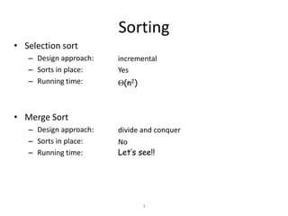
n1 n2](https://image.slidesharecdn.com/mergesortandquicksort-140701050833-phpapp01/85/Merge-sort-and-quick-sort-11-320.jpg)
![Algorithm:
mergesort( int [] a, int left, int right)
{
if (right > left)
{ middle = left + (right - left)/2;
mergesort(a, left, middle);
mergesort(a, middle+1, right);
merge(a, left, middle, right); }
}
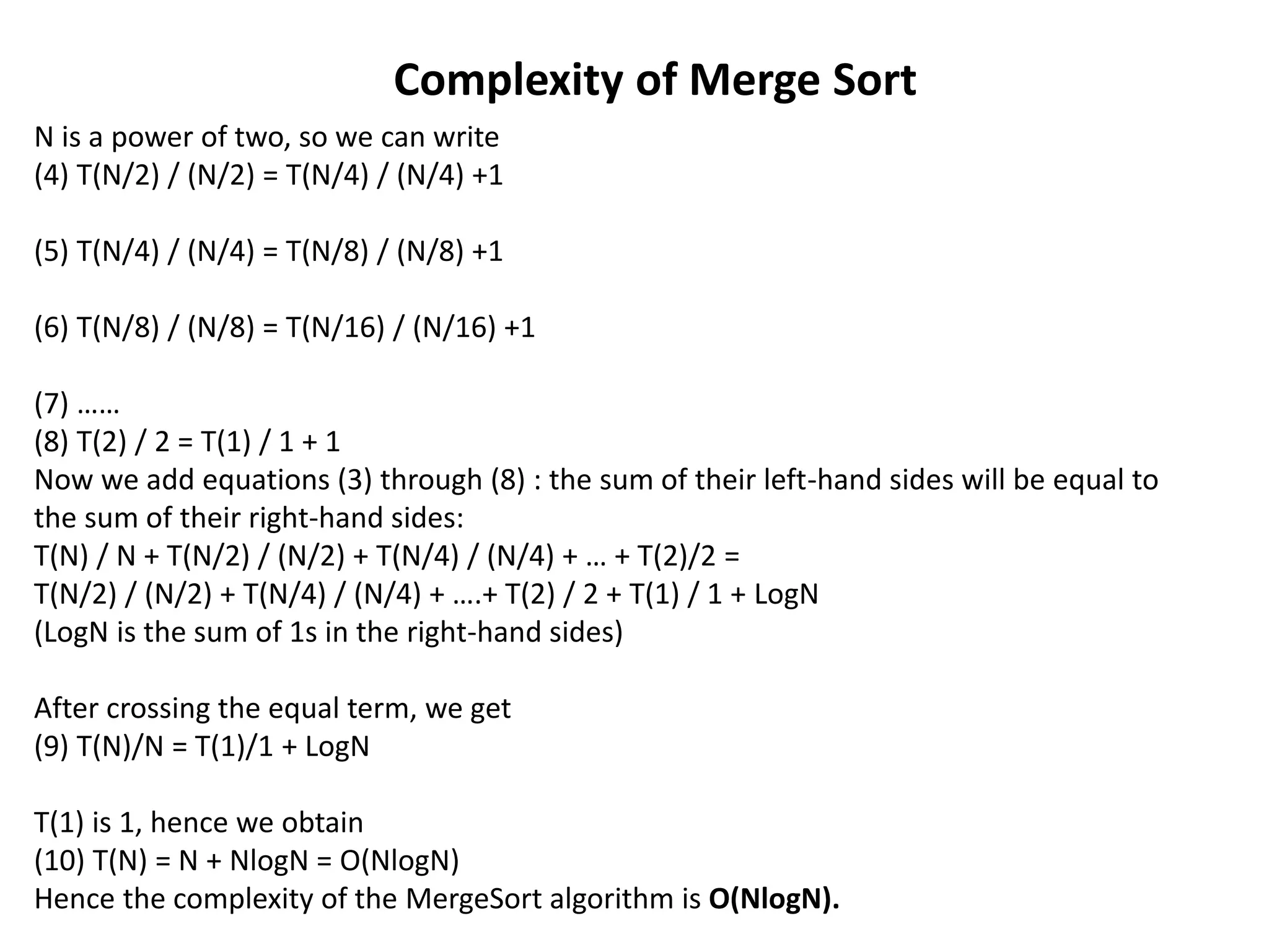
Assumption: N is a power of two. For N = 1: time is a constant (denoted by 1)
Otherwise, time to mergesort N elements = time to mergesort N/2 elements + time to merge
two arrays each N/2 elements.
Time to merge two arrays each N/2 elements is linear, i.e. N
Thus we have:
(1) T(1) = 1
(2) T(N) = 2T(N/2) + N
Next we will solve this recurrence relation. First we divide (2) by N:
(3) T(N) / N = T(N/2) / (N/2) + 1
Complexity of Merge Sort](https://image.slidesharecdn.com/mergesortandquicksort-140701050833-phpapp01/85/Merge-sort-and-quick-sort-12-320.jpg)

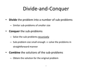
![14
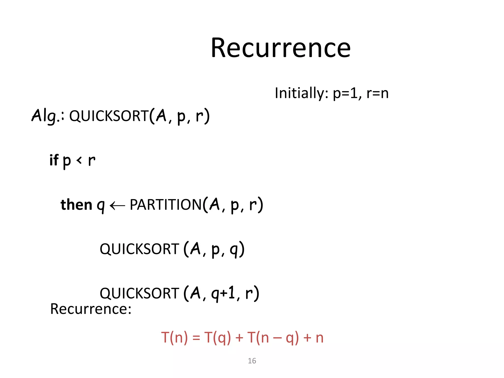
Quicksort
• Sort an array A[p…r]
• Divide
– Partition the array A into 2 subarrays A[p..q] and A[q+1..r], such that
each element of A[p..q] is smaller than or equal to each element in
A[q+1..r]
– Need to find index q to partition the array
≤A[p…q] A[q+1…r]](https://image.slidesharecdn.com/mergesortandquicksort-140701050833-phpapp01/85/Merge-sort-and-quick-sort-14-320.jpg)
![15
Quicksort
• Conquer
– Recursively sort A[p..q] and A[q+1..r] using Quicksort
• Combine
– Trivial: the arrays are sorted in place
– No additional work is required to combine them
– The entire array is now sorted
A[p…q] A[q+1…r]≤](https://image.slidesharecdn.com/mergesortandquicksort-140701050833-phpapp01/85/Merge-sort-and-quick-sort-15-320.jpg)

![17
Partitioning the Array
Alg. PARTITION (A, p, r)
1. x A[p]
2. i p – 1
3. j r + 1
4. while TRUE
5. do repeat j j – 1
6. until A[j] ≤ x
7. do repeat i i + 1
8. until A[i] ≥ x
9. if i < j
10. then exchange A[i] A[j]
11. else return j
Running time: (n)
n = r – p + 1
73146235
i j
A:
arap
ij=q
A:
A[p…q] A[q+1…r]≤
p r
Each element is
visited once!](https://image.slidesharecdn.com/mergesortandquicksort-140701050833-phpapp01/85/Merge-sort-and-quick-sort-17-320.jpg)


![5
Merge Sort Approach
• To sort an array A[p . . r]:
• Divide
– Divide the n-element sequence to be sorted into two
subsequences of n/2 elements each
• Conquer
– Sort the subsequences recursively using merge sort
– When the size of the sequences is 1 there is nothing
more to do
• Combine
– Merge the two sorted subsequences](https://image.slidesharecdn.com/mergesortandquicksort-140701050833-phpapp01/75/Merge-sort-and-quick-sort-5-2048.jpg)

![11
Merge - Pseudocode
Alg.: MERGE(A, p, q, r)
1. Compute n1 and n2
2. Copy the first n1 elements into L[1
. . n1 + 1] and the next n2 elements into R[1 . . n2 + 1]
3. L[n1 + 1] ← ; R[n2 + 1] ←
4. i ← 1; j ← 1
5. for k ← p to r
6. do if L[ i ] ≤ R[ j ]
7. then A[k] ← L[ i ]
8. i ←i + 1
9. else A[k] ← R[ j ]
10. j ← j + 1
p q
7542
6321
rq + 1
L
R
1 2 3 4 5 6 7 8
63217542
p rq
n1 n2](https://image.slidesharecdn.com/mergesortandquicksort-140701050833-phpapp01/75/Merge-sort-and-quick-sort-11-2048.jpg)
![Algorithm:
mergesort( int [] a, int left, int right)
{
if (right > left)
{ middle = left + (right - left)/2;
mergesort(a, left, middle);
mergesort(a, middle+1, right);
merge(a, left, middle, right); }
}
Assumption: N is a power of two. For N = 1: time is a constant (denoted by 1)
Otherwise, time to mergesort N elements = time to mergesort N/2 elements + time to merge
two arrays each N/2 elements.
Time to merge two arrays each N/2 elements is linear, i.e. N
Thus we have:
(1) T(1) = 1
(2) T(N) = 2T(N/2) + N
Next we will solve this recurrence relation. First we divide (2) by N:
(3) T(N) / N = T(N/2) / (N/2) + 1
Complexity of Merge Sort](https://image.slidesharecdn.com/mergesortandquicksort-140701050833-phpapp01/75/Merge-sort-and-quick-sort-12-2048.jpg)
![14
Quicksort
• Sort an array A[p…r]
• Divide
– Partition the array A into 2 subarrays A[p..q] and A[q+1..r], such that
each element of A[p..q] is smaller than or equal to each element in
A[q+1..r]
– Need to find index q to partition the array
≤A[p…q] A[q+1…r]](https://image.slidesharecdn.com/mergesortandquicksort-140701050833-phpapp01/75/Merge-sort-and-quick-sort-14-2048.jpg)
![15
Quicksort
• Conquer
– Recursively sort A[p..q] and A[q+1..r] using Quicksort
• Combine
– Trivial: the arrays are sorted in place
– No additional work is required to combine them
– The entire array is now sorted
A[p…q] A[q+1…r]≤](https://image.slidesharecdn.com/mergesortandquicksort-140701050833-phpapp01/75/Merge-sort-and-quick-sort-15-2048.jpg)
![17
Partitioning the Array
Alg. PARTITION (A, p, r)
1. x A[p]
2. i p – 1
3. j r + 1
4. while TRUE
5. do repeat j j – 1
6. until A[j] ≤ x
7. do repeat i i + 1
8. until A[i] ≥ x
9. if i < j
10. then exchange A[i] A[j]
11. else return j
Running time: (n)
n = r – p + 1
73146235
i j
A:
arap
ij=q
A:
A[p…q] A[q+1…r]≤
p r
Each element is
visited once!](https://image.slidesharecdn.com/mergesortandquicksort-140701050833-phpapp01/75/Merge-sort-and-quick-sort-17-2048.jpg)

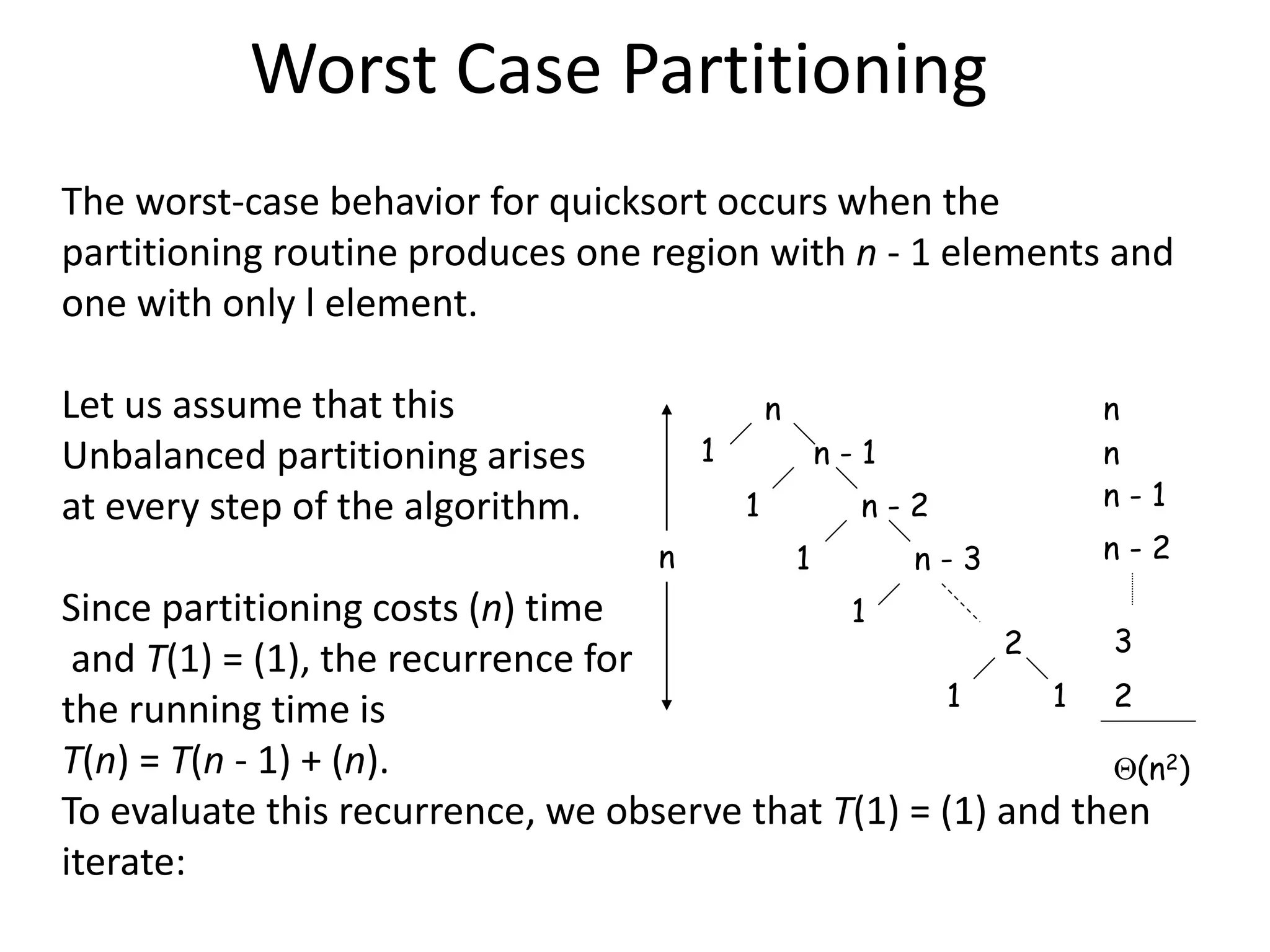
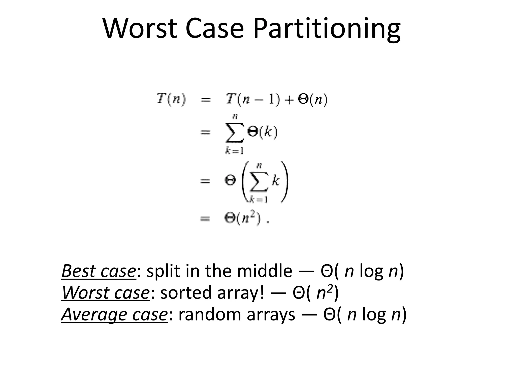

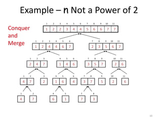
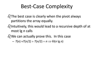
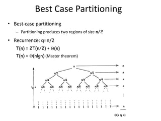
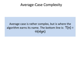
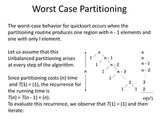
The document discusses different sorting algorithms including merge sort and quicksort. Merge sort has a divide and conquer approach where an array is divided into halves and the halves are merged back together in sorted order. This results in a runtime of O(n log n). Quicksort uses a partitioning approach, choosing a pivot element and partitioning the array into subarrays of elements less than or greater than the pivot. In the best case, this partitions the array in half at each step, resulting in a runtime of O(n log n). In the average case, the runtime is also O(n log n). In the worst case, the array is already sorted, resulting in unbalanced partitions and a quadratic runtime of O(n^2
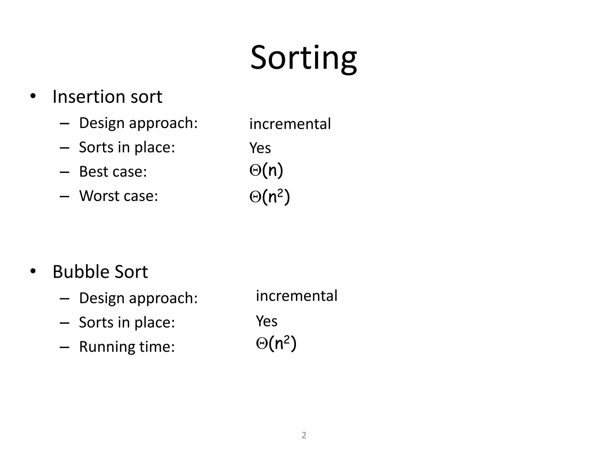
Introduction to various sorting algorithms: Insertion, Bubble, Selection, Merge Sort; their design approaches and time complexities.
Explanation of Divide-and-Conquer strategy: dividing problem, solving subproblems recursively, and combining solutions.
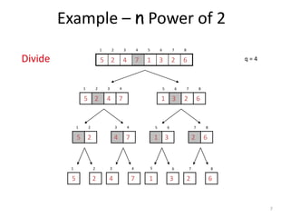
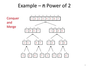
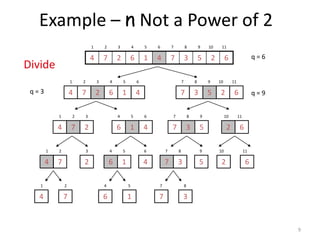
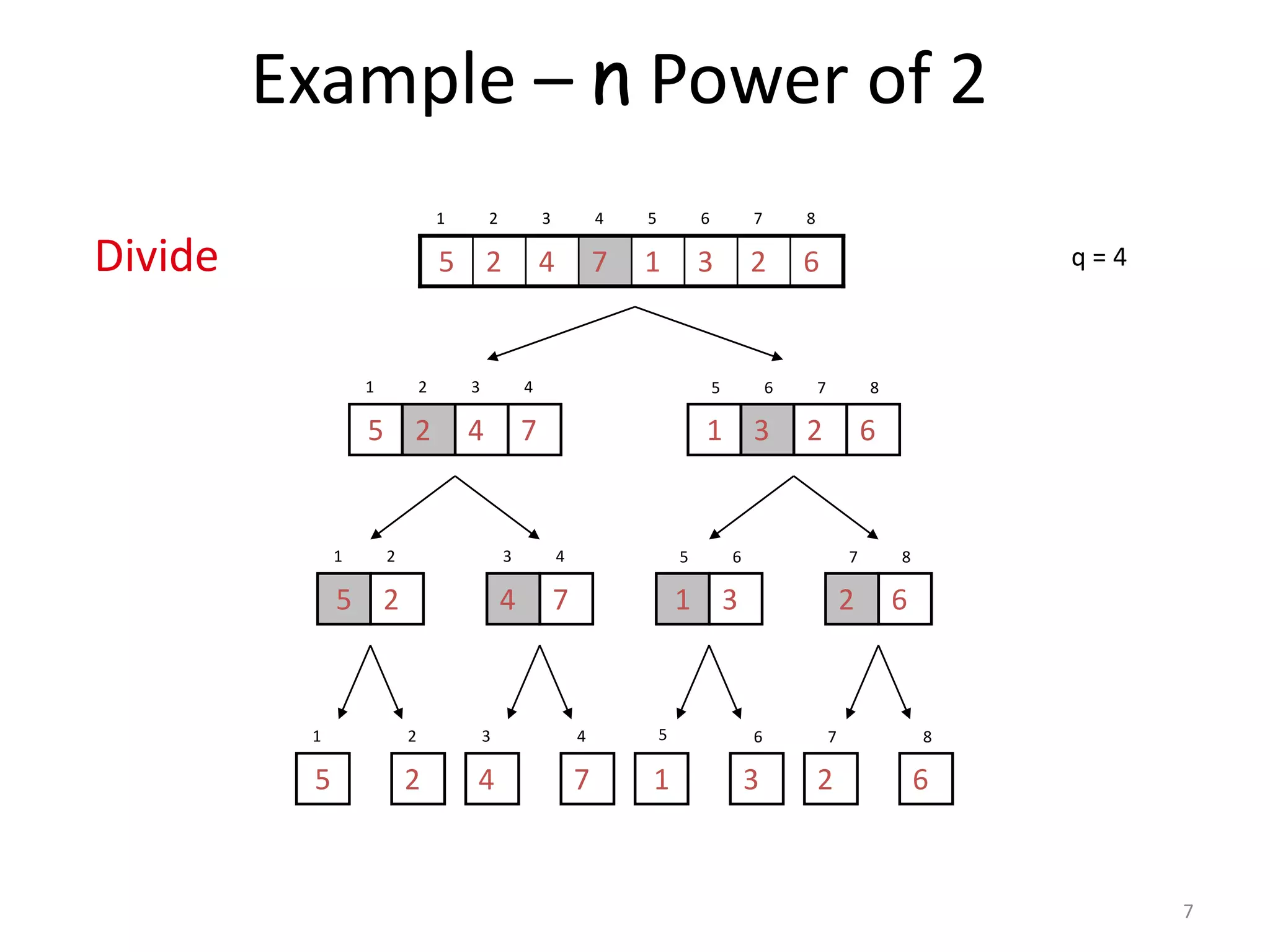
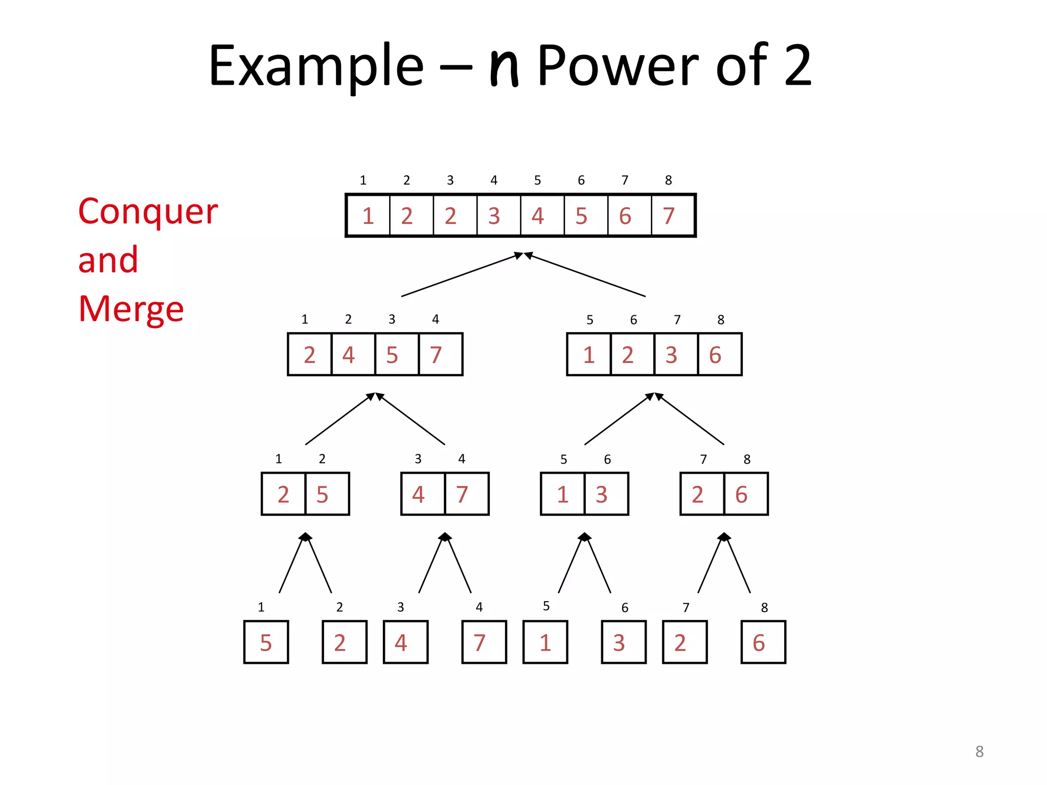
Details on Merge Sort: dividing array, recursive sorting, and merging sorted subsequences with examples.
Pseudocode for Merge Sort, merging arrays, and example arrays showcasing merge operations.
Analysis of Merge Sort time complexity derivation showing O(N log N) using recurrence relations.
Overview of Quicksort: partitioning the array, recursive sorting, and the trivial combining stage.
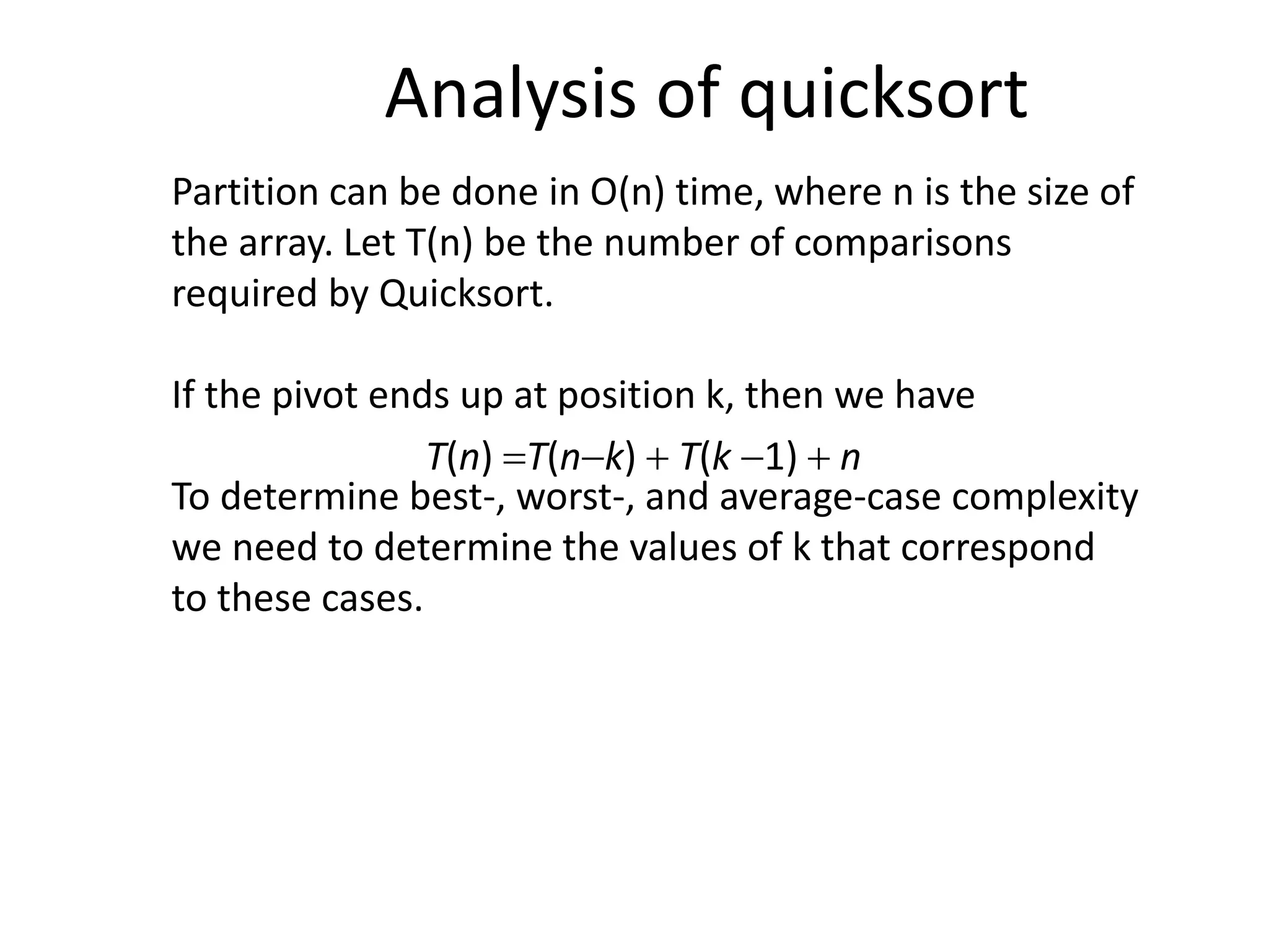
Details on the partitioning algorithm for Quicksort and its time complexity analysis.
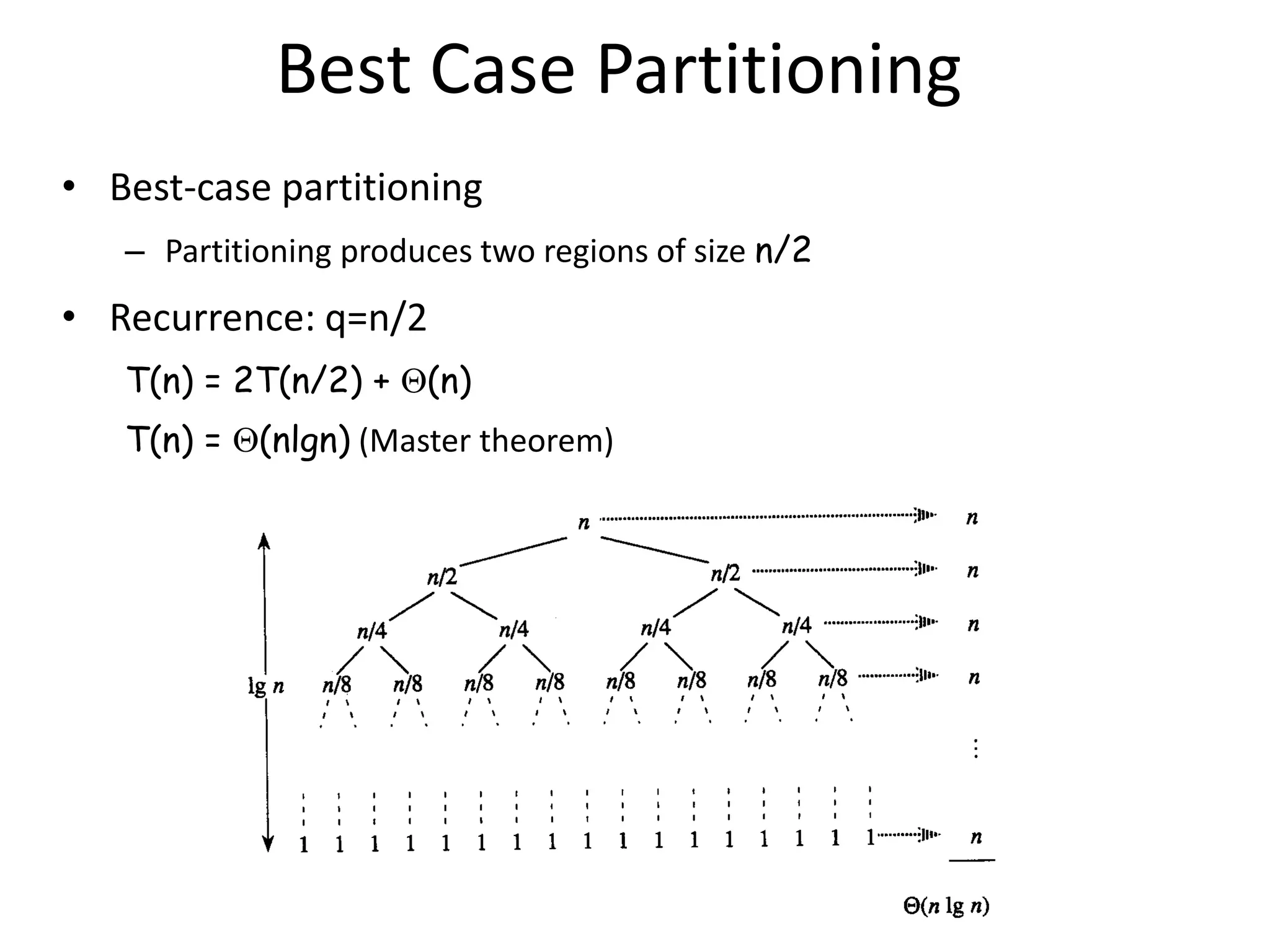
Best, average, and worst-case complexities of Quicksort, proving each case using recurrence relations.


![Data Structures - Lecture 8 [Sorting Algorithms]](https://cdn.slidesharecdn.com/ss_thumbnails/lecture-8sortingalgorithms-150205105023-conversion-gate02-thumbnail.jpg?width=600ounds&width=560&fit=bounds)


