Download to read offline
![Sequential Search
Algorithm SequentialSearch(A[0…n-1], K)
//Problem Description: Searches for a given value in a given array by
// sequential search
//Input: An Array A[0…n-1] and a search key K
//Output: Returns the index of the first element of A that matches K
// or -1 if there are no matching elements
i 0
while i < n and A[i] K do
i i+1
if i < n return i
else return -1
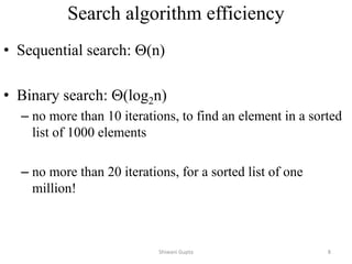
1. Worst case: O(n)
2. Best case: O(1)
3. Average case: O(n/2)
Thus, we say sequential search is O(n)
Shiwani Gupta 4](https://image.slidesharecdn.com/module2dividenconquer2022-220810034536-bde42288/85/module2_dIVIDEncONQUER_2022-pdf-4-320.jpg)
![Binary Search: pseudo-code (ITERATIVE)
binary_search(a, x)
left ← 0
right ← N-1
while(left <= right)
mid= (left+right)/2
if (a[mid] > x)
right ← mid – 1
else if (x > a[mid])
low ← mid + 1
else
return mid //found
return -1 //not found
Shiwani Gupta 6](https://image.slidesharecdn.com/module2dividenconquer2022-220810034536-bde42288/85/module2_dIVIDEncONQUER_2022-pdf-6-320.jpg)
![Binary Search: pseudo-code (RECURSIVE)
binary_search(a, x, left, right)
if (right < left)
return -1 // not found
mid= floor((left+right)/2) //floor(.)=(int)(.)
if (a[mid] == x)
return mid
else if (x < a[mid])
binary_search(a, x, left, mid-1)
else
binary_search(a, x, mid+1, right)
Binary Search: Time Complexity (for successful search)
Number of comparisons:
T(n) = T(n/2) + 1, if n>1;
= 1, if n=1
which solves to T(n) = Ѳ(logn) with Case 2 of Master Method. 7](https://image.slidesharecdn.com/module2dividenconquer2022-220810034536-bde42288/85/module2_dIVIDEncONQUER_2022-pdf-7-320.jpg)
![Finding Max Min
StraightMaxMin(a, n, max, min)
max = min = a[1]
for i = 2 to n do
if (a[i]>max) then max = a[i] //n-1 comparisons
if (a[i]<min) then min = a[i] //n-1 comparisons
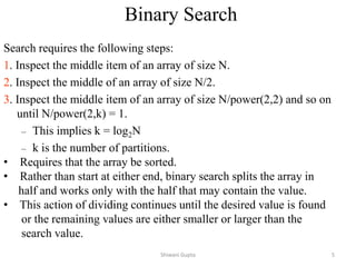
Total = 2*(n-1) comparisons
1. Worst case: O(n)
2. Best case: O(n)
3. Average case: O(n)
Thus, we say Straight Max Min is O(n).
Shiwani Gupta 9](https://image.slidesharecdn.com/module2dividenconquer2022-220810034536-bde42288/85/module2_dIVIDEncONQUER_2022-pdf-9-320.jpg)
![MaxMin(i,j,max,min) //1<=i<=j<=n
if ( i == j) then max = min = a[i] //single element
else if (i == j -1) then //two elements
if (a[i] < a[j]) then
max = a[j]
min = a[i]
else
max = a[i]
min = a[j]
else //divide P into subproblems
mid = (i+j)/2 //find split
MaxMin(i, mid, max, min) //solve subproblems
MaxMin(mid+1, j, max1, min1) //solve subproblems
if (max<max1) then max = max1 //combine solutions
if (min>min1) then min = min1 //combine solutions
The recurrence for this algorithm is
T(n) = 2T(n/2) + 2 n>2 when
max and min are considered as different procedures
T(n) = 1 n=2
T(n) = 0 n=1
This solves to T(n) = 3n/2-2.
Finding Max Min
10](https://image.slidesharecdn.com/module2dividenconquer2022-220810034536-bde42288/85/module2_dIVIDEncONQUER_2022-pdf-10-320.jpg)


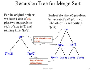
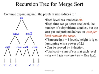
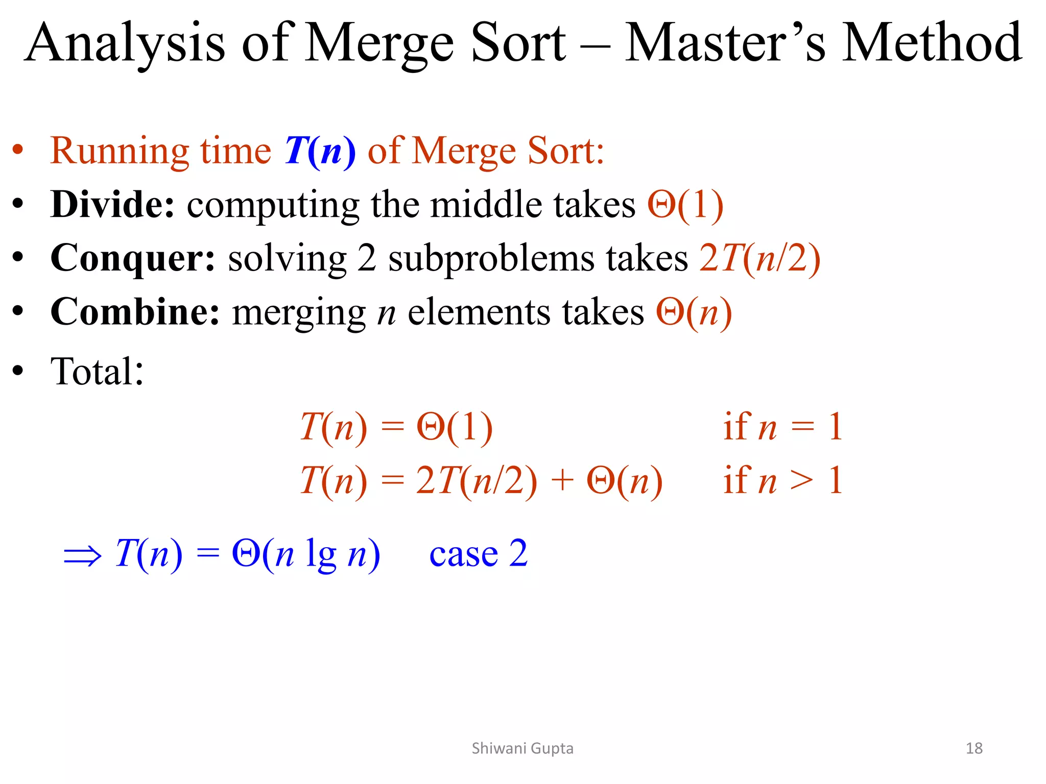
![Merge-Sort (A, p, r)
INPUT: a sequence of n numbers stored in array A
OUTPUT: an ordered sequence of n numbers
MergeSort (A, p, r) // p as beginning pointer of array and r as end pointer
1 if p < r
2 then q (p+r)/2 //split the list at mid
3 MergeSort (A, p, q) //first sublist
4 MergeSort (A, q+1, r) //second sublist
5 Merge (A, p, q, r) // merges A[p..q] with A[q+1..r]
Initial Call: MergeSort(A, 1, n)
Shiwani Gupta 15](https://image.slidesharecdn.com/module2dividenconquer2022-220810034536-bde42288/85/module2_dIVIDEncONQUER_2022-pdf-14-320.jpg)
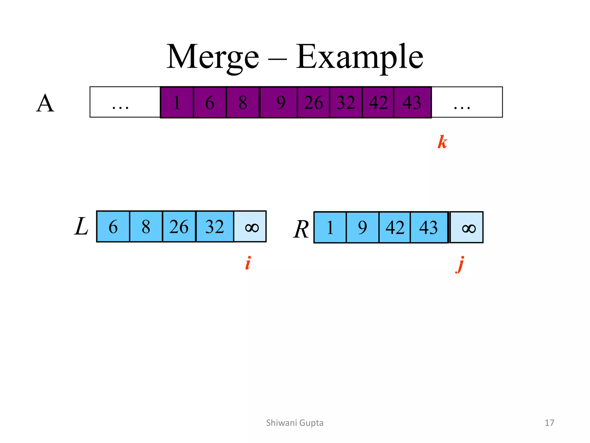
![Procedure Merge
Merge(A, p, q, r)
1 n1 q – p + 1
2 n2 r – q
3 for i 1 to n1
4 do L[i] A[p + i – 1]
5 for j 1 to n2
6 do R[j] A[q + j]
7 L[n1+1]
8 R[n2+1]
9 i 1
10 j 1
11 for k p to r
12 do if L[i] R[j]
13 then A[k] L[i]
14 i i + 1
15 else A[k] R[j]
16 j j + 1
Sentinels, to avoid having to
check if either subarray is
fully copied at each step.
Input: Array containing sorted
subarrays A[p..q] and
A[q+1..r].
Output: Merged sorted
subarray in A[p..r].
Shiwani Gupta 16](https://image.slidesharecdn.com/module2dividenconquer2022-220810034536-bde42288/85/module2_dIVIDEncONQUER_2022-pdf-15-320.jpg)


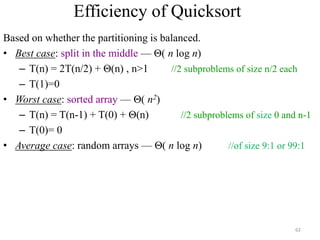
![Quicksort
• Divide: Partition array A[l..r] into 2 subarrays, A[l..s-1] and
A[s+1..r] such that each element of the first array is ≤ A[s]
and each element of the second array is ≥ A[s]. (computing
the index of s is part of partition.)
– Implication: A[s] will be in its final position in the sorted
array.
• Conquer: Sort the two subarrays A[l..s-1] and A[s+1..r] by
recursive calls to Quicksort
• Combine: No work is needed, because A[s] is already in its
correct place after the partition is done, and the two
subarrays have been sorted.
Shiwani Gupta 23](https://image.slidesharecdn.com/module2dividenconquer2022-220810034536-bde42288/85/module2_dIVIDEncONQUER_2022-pdf-22-320.jpg)
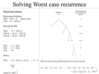
![The Quicksort Algorithm
ALGORITHM Quicksort(A[l..r])
//Problem Description: Sorts a subarray by quicksort
//Input: A subarray A[l..r] of A[0..n-1],defined by its left and right
indices l and r
//Output: The subarray A[l..r] sorted in nondecreasing order
if l < r
s Partition (A[l..r]) // s is a split position
Quicksort(A[l..s-1])
Quicksort(A[s+1..r]
Shiwani Gupta 24](https://image.slidesharecdn.com/module2dividenconquer2022-220810034536-bde42288/85/module2_dIVIDEncONQUER_2022-pdf-23-320.jpg)
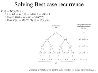
![Partitioning Algorithm
Algorithm Partition(A[l, r])
p A[l ]
i l; j r+1
repeat
repeat i←i+1 until A[i]>p
repeat j←j-1 until A[i]<=p
swap(A[i],A[j])
until i>j
swap(p,A[j])
Shiwani Gupta 25](https://image.slidesharecdn.com/module2dividenconquer2022-220810034536-bde42288/85/module2_dIVIDEncONQUER_2022-pdf-24-320.jpg)
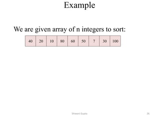
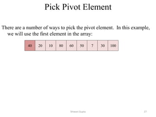
![40 20 10 80 60 50 7 30 100
p = 0
[0] [1] [2] [3] [4] [5] [6] [7] [8]
i j
Shiwani Gupta 28](https://image.slidesharecdn.com/module2dividenconquer2022-220810034536-bde42288/85/module2_dIVIDEncONQUER_2022-pdf-27-320.jpg)
![40 20 10 80 60 50 7 30 100
[0] [1] [2] [3] [4] [5] [6] [7] [8]
i j
1. while data[i] <= data[p]
++i
p = 0
Shiwani Gupta 29](https://image.slidesharecdn.com/module2dividenconquer2022-220810034536-bde42288/85/module2_dIVIDEncONQUER_2022-pdf-28-320.jpg)
![40 20 10 80 60 50 7 30 100
[0] [1] [2] [3] [4] [5] [6] [7] [8]
i j
1. while data[i] <= data[p]
++i
p = 0
Shiwani Gupta 30](https://image.slidesharecdn.com/module2dividenconquer2022-220810034536-bde42288/85/module2_dIVIDEncONQUER_2022-pdf-29-320.jpg)
![40 20 10 80 60 50 7 30 100
[0] [1] [2] [3] [4] [5] [6] [7] [8]
i j
1. while data[i] <= data[p]
++i
p = 0
Shiwani Gupta 31](https://image.slidesharecdn.com/module2dividenconquer2022-220810034536-bde42288/85/module2_dIVIDEncONQUER_2022-pdf-30-320.jpg)
![40 20 10 80 60 50 7 30 100
[0] [1] [2] [3] [4] [5] [6] [7] [8]
i j
1. while data[i] <= data[p]
++i
2. while data[j] > data[p]
--j
p = 0
Shiwani Gupta 32](https://image.slidesharecdn.com/module2dividenconquer2022-220810034536-bde42288/85/module2_dIVIDEncONQUER_2022-pdf-31-320.jpg)
![40 20 10 80 60 50 7 30 100
[0] [1] [2] [3] [4] [5] [6] [7] [8]
i j
1. while data[i] <= data[p]
++i
2. while data[j] > data[p]
--j
p = 0
Shiwani Gupta 33](https://image.slidesharecdn.com/module2dividenconquer2022-220810034536-bde42288/85/module2_dIVIDEncONQUER_2022-pdf-32-320.jpg)
![40 20 10 80 60 50 7 30 100
[0] [1] [2] [3] [4] [5] [6] [7] [8]
i j
1. while data[i] <= data[p]
++i
2. while data[j] > data[p]
--j
3. if i < j
swap data[i] and data[j]
p = 0
Shiwani Gupta 34](https://image.slidesharecdn.com/module2dividenconquer2022-220810034536-bde42288/85/module2_dIVIDEncONQUER_2022-pdf-33-320.jpg)
![40 20 10 30 60 50 7 80 100
[0] [1] [2] [3] [4] [5] [6] [7] [8]
i j
1. while data[i] <= data[p]
++i
2. while data[j] > data[p]
--j
3. if i < j
swap data[i] and data[j]
p = 0
Shiwani Gupta 35](https://image.slidesharecdn.com/module2dividenconquer2022-220810034536-bde42288/85/module2_dIVIDEncONQUER_2022-pdf-34-320.jpg)
![40 20 10 30 60 50 7 80 100
[0] [1] [2] [3] [4] [5] [6] [7] [8]
i j
1. while data[i] <= data[p]
++i
2. while data[j] > data[p]
--j
3. if i < j
swap data[i] and data[j]
4. while j > i, go to 1.
p = 0
Shiwani Gupta 36](https://image.slidesharecdn.com/module2dividenconquer2022-220810034536-bde42288/85/module2_dIVIDEncONQUER_2022-pdf-35-320.jpg)
![40 20 10 30 60 50 7 80 100
[0] [1] [2] [3] [4] [5] [6] [7] [8]
i j
1. while data[i] <= data[p]
++i
2. while data[j] > data[p]
--j
3. if i < j
swap data[i] and data[j]
4. while j > i, go to 1.
p = 0
Shiwani Gupta 37](https://image.slidesharecdn.com/module2dividenconquer2022-220810034536-bde42288/85/module2_dIVIDEncONQUER_2022-pdf-36-320.jpg)
![40 20 10 30 60 50 7 80 100
[0] [1] [2] [3] [4] [5] [6] [7] [8]
i j
1. while data[i] <= data[p]
++i
2. while data[j] > data[p]
--j
3. if i < j
swap data[i] and data[j]
4. while j > i, go to 1.
p = 0
Shiwani Gupta 38](https://image.slidesharecdn.com/module2dividenconquer2022-220810034536-bde42288/85/module2_dIVIDEncONQUER_2022-pdf-37-320.jpg)
![40 20 10 30 60 50 7 80 100
[0] [1] [2] [3] [4] [5] [6] [7] [8]
i j
1. while data[i] <= data[p]
++i
2. while data[j] > data[p]
--j
3. if i < j
swap data[i] and data[j]
4. while j > i, go to 1.
p = 0
Shiwani Gupta 39](https://image.slidesharecdn.com/module2dividenconquer2022-220810034536-bde42288/85/module2_dIVIDEncONQUER_2022-pdf-38-320.jpg)
![40 20 10 30 60 50 7 80 100
[0] [1] [2] [3] [4] [5] [6] [7] [8]
i j
1. while data[i] <= data[p]
++i
2. while data[j] > data[p]
--j
3. if i < j
swap data[i] and data[j]
4. while j > i, go to 1.
p = 0
Shiwani Gupta 40](https://image.slidesharecdn.com/module2dividenconquer2022-220810034536-bde42288/85/module2_dIVIDEncONQUER_2022-pdf-39-320.jpg)
![40 20 10 30 60 50 7 80 100
[0] [1] [2] [3] [4] [5] [6] [7] [8]
i j
1. while data[i] <= data[p]
++i
2. while data[j] > data[p]
--j
3. if i < j
swap data[i] and data[j]
4. while j > i, go to 1.
p = 0
Shiwani Gupta 41](https://image.slidesharecdn.com/module2dividenconquer2022-220810034536-bde42288/85/module2_dIVIDEncONQUER_2022-pdf-40-320.jpg)
![1. while data[i] <= data[p]
++i
2. while data[j] > data[p]
--j
3. if i < j
swap data[i] and data[j]
4. while j > i, go to 1.
40 20 10 30 7 50 60 80 100
[0] [1] [2] [3] [4] [5] [6] [7] [8]
i j
p = 0
Shiwani Gupta 42](https://image.slidesharecdn.com/module2dividenconquer2022-220810034536-bde42288/85/module2_dIVIDEncONQUER_2022-pdf-41-320.jpg)
![1. while data[i] <= data[p]
++i
2. while data[j] > data[p]
--j
3. if i < j
swap data[i] and data[j]
4. while j > i, go to 1.
40 20 10 30 7 50 60 80 100
[0] [1] [2] [3] [4] [5] [6] [7] [8]
i j
p = 0
Shiwani Gupta 43](https://image.slidesharecdn.com/module2dividenconquer2022-220810034536-bde42288/85/module2_dIVIDEncONQUER_2022-pdf-42-320.jpg)
![1. while data[i] <= data[p]
++i
2. while data[j] > data[p]
--j
3. if i < j
swap data[i] and data[j]
4. while j > i, go to 1.
40 20 10 30 7 50 60 80 100
[0] [1] [2] [3] [4] [5] [6] [7] [8]
i j
p = 0
Shiwani Gupta 44](https://image.slidesharecdn.com/module2dividenconquer2022-220810034536-bde42288/85/module2_dIVIDEncONQUER_2022-pdf-43-320.jpg)
![1. while data[i] <= data[p]
++i
2. while data[j] > data[p]
--j
3. if i < j
swap data[i] and data[j]
4. while j > i, go to 1.
40 20 10 30 7 50 60 80 100
[0] [1] [2] [3] [4] [5] [6] [7] [8]
i j
p = 0
Shiwani Gupta 45](https://image.slidesharecdn.com/module2dividenconquer2022-220810034536-bde42288/85/module2_dIVIDEncONQUER_2022-pdf-44-320.jpg)
![1. while data[i] <= data[p]
++i
2. while data[j] > data[p]
--j
3. if i < j
swap data[i] and data[j]
4. while j > i, go to 1.
40 20 10 30 7 50 60 80 100
[0] [1] [2] [3] [4] [5] [6] [7] [8]
i j
p = 0
Shiwani Gupta 46](https://image.slidesharecdn.com/module2dividenconquer2022-220810034536-bde42288/85/module2_dIVIDEncONQUER_2022-pdf-45-320.jpg)
![1. while data[i] <= data[p]
++i
2. while data[j] > data[p]
--j
3. if i < j
swap data[i] and data[j]
4. while j > i, go to 1.
40 20 10 30 7 50 60 80 100
[0] [1] [2] [3] [4] [5] [6] [7] [8]
i j
p = 0
Shiwani Gupta 47](https://image.slidesharecdn.com/module2dividenconquer2022-220810034536-bde42288/85/module2_dIVIDEncONQUER_2022-pdf-46-320.jpg)
![1. while data[i] <= data[p]
++i
2. while data[j] > data[p]
--j
3. if i < j
swap data[i] and data[j]
4. while j > i, go to 1.
40 20 10 30 7 50 60 80 100
[0] [1] [2] [3] [4] [5] [6] [7] [8]
i j
p = 0
Shiwani Gupta 48](https://image.slidesharecdn.com/module2dividenconquer2022-220810034536-bde42288/85/module2_dIVIDEncONQUER_2022-pdf-47-320.jpg)
![1. while data[i] <= data[p]
++i
2. while data[j] > data[p]
--j
3. if i < j
swap data[i] and data[j]
4. while j > i, go to 1.
40 20 10 30 7 50 60 80 100
p = 0
[0] [1] [2] [3] [4] [5] [6] [7] [8]
i j
Shiwani Gupta 49](https://image.slidesharecdn.com/module2dividenconquer2022-220810034536-bde42288/85/module2_dIVIDEncONQUER_2022-pdf-48-320.jpg)
![1. while data[i] <= data[p]
++i
2. while data[j] > data[p]
--j
3. if i < j
swap data[i] and data[j]
4. while j > i, go to 1.
40 20 10 30 7 50 60 80 100
p = 0
[0] [1] [2] [3] [4] [5] [6] [7] [8]
i j
Shiwani Gupta 50](https://image.slidesharecdn.com/module2dividenconquer2022-220810034536-bde42288/85/module2_dIVIDEncONQUER_2022-pdf-49-320.jpg)
![1. while data[i] <= data[p]
++i
2. while data[j] > data[p]
--j
3. if i < j
swap data[i] and data[j]
4. while j > i, go to 1.
5. swap data[j] and data[p]
40 20 10 30 7 50 60 80 100
p = 0
[0] [1] [2] [3] [4] [5] [6] [7] [8]
i j
Shiwani Gupta 51](https://image.slidesharecdn.com/module2dividenconquer2022-220810034536-bde42288/85/module2_dIVIDEncONQUER_2022-pdf-50-320.jpg)
![1. while data[i] <= data[p]
++i
2. while data[j] > data[p]
--j
3. if i < j
swap data[i] and data[j]
4. while j > i, go to 1.
5. swap data[j] and data[p]
7 20 10 30 40 50 60 80 100
p = 4
[0] [1] [2] [3] [4] [5] [6] [7] [8]
i j
Shiwani Gupta 52](https://image.slidesharecdn.com/module2dividenconquer2022-220810034536-bde42288/85/module2_dIVIDEncONQUER_2022-pdf-51-320.jpg)
![7 20 10 30 40 50 60 80 100
[0] [1] [2] [3] [4] [5] [6] [7] [8]
<= data[p] > data[p]
Partition Result
Best Case
Shiwani Gupta 53](https://image.slidesharecdn.com/module2dividenconquer2022-220810034536-bde42288/85/module2_dIVIDEncONQUER_2022-pdf-52-320.jpg)
![Quicksort: Worst Case
• Assume first element is chosen as p.
• Assume we get array that is already in order:
2 4 10 12 13 50 57 63 100
p = 0
[0] [1] [2] [3] [4] [5] [6] [7] [8]
i j
Shiwani Gupta 54](https://image.slidesharecdn.com/module2dividenconquer2022-220810034536-bde42288/85/module2_dIVIDEncONQUER_2022-pdf-53-320.jpg)
![1. while data[i] <= data[p]
++i
2. while data[j] > data[p]
--j
3. if i < j
swap data[i] and data[j]
4. while j > i, go to 1.
5. swap data[j] and data[p]
2 4 10 12 13 50 57 63 100
p = 0
[0] [1] [2] [3] [4] [5] [6] [7] [8]
i j
Shiwani Gupta 55](https://image.slidesharecdn.com/module2dividenconquer2022-220810034536-bde42288/85/module2_dIVIDEncONQUER_2022-pdf-54-320.jpg)
![1. while data[i] <= data[p]
++i
2. while data[j] > data[p]
--j
3. if i < j
swap data[i] and data[j]
4. while j > i, go to 1.
5. swap data[j] and data[p]
2 4 10 12 13 50 57 63 100
p = 0
[0] [1] [2] [3] [4] [5] [6] [7] [8]
i j
Shiwani Gupta 56](https://image.slidesharecdn.com/module2dividenconquer2022-220810034536-bde42288/85/module2_dIVIDEncONQUER_2022-pdf-55-320.jpg)
![1. while data[i] <= data[p]
++i
2. while data[j] > data[p]
--j
3. if i < j
swap data[i] and data[j]
4. while j > i, go to 1.
5. swap data[j] and data[p]
2 4 10 12 13 50 57 63 100
p = 0
[0] [1] [2] [3] [4] [5] [6] [7] [8]
i j
Shiwani Gupta 57](https://image.slidesharecdn.com/module2dividenconquer2022-220810034536-bde42288/85/module2_dIVIDEncONQUER_2022-pdf-56-320.jpg)
![1. while data[i] <= data[p]
++i
2. while data[j] > data[p]
--j
3. if i < j
swap data[i] and data[j]
4. while j > i, go to 1.
5. swap data[j] and data[p]
2 4 10 12 13 50 57 63 100
p = 0
[0] [1] [2] [3] [4] [5] [6] [7] [8]
i j
Shiwani Gupta 58](https://image.slidesharecdn.com/module2dividenconquer2022-220810034536-bde42288/85/module2_dIVIDEncONQUER_2022-pdf-57-320.jpg)
![1. while data[i] <= data[p]
++i
2. while data[j] > data[p]
--j
3. if i < j
swap data[i] and data[j]
4. while j > i, go to 1.
5. swap data[j] and data[p]
2 4 10 12 13 50 57 63 100
p = 0
[0] [1] [2] [3] [4] [5] [6] [7] [8]
i j
Shiwani Gupta 59](https://image.slidesharecdn.com/module2dividenconquer2022-220810034536-bde42288/85/module2_dIVIDEncONQUER_2022-pdf-58-320.jpg)
![1. While data[i] <= data[p]
++i
2. While data[j] > data[p]
--j
3. If i < j
swap data[i] and data[j]
4. While j > i, go to 1.
5. Swap data[j] and data[p]
2 4 10 12 13 50 57 63 100
p = 0
[0] [1] [2] [3] [4] [5] [6] [7] [8]
i j
Shiwani Gupta 60](https://image.slidesharecdn.com/module2dividenconquer2022-220810034536-bde42288/85/module2_dIVIDEncONQUER_2022-pdf-59-320.jpg)
![1. While data[i] <= data[p]
++i
2. While data[j] > data[p]
--j
3. If i < j
swap data[i] and data[j]
4. While j > i, go to 1.
5. Swap data[j] and data[p]
2 4 10 12 13 50 57 63 100
p = 0
[0] [1] [2] [3] [4] [5] [6] [7] [8]
> data[p]
<= data[p]
Shiwani Gupta 61](https://image.slidesharecdn.com/module2dividenconquer2022-220810034536-bde42288/85/module2_dIVIDEncONQUER_2022-pdf-60-320.jpg)

![Sequential Search
Algorithm SequentialSearch(A[0…n-1], K)
//Problem Description: Searches for a given value in a given array by
// sequential search
//Input: An Array A[0…n-1] and a search key K
//Output: Returns the index of the first element of A that matches K
// or -1 if there are no matching elements
i 0
while i < n and A[i] K do
i i+1
if i < n return i
else return -1
1. Worst case: O(n)
2. Best case: O(1)
3. Average case: O(n/2)
Thus, we say sequential search is O(n)
Shiwani Gupta 4](https://image.slidesharecdn.com/module2dividenconquer2022-220810034536-bde42288/75/module2_dIVIDEncONQUER_2022-pdf-4-2048.jpg)
![Binary Search: pseudo-code (ITERATIVE)
binary_search(a, x)
left ← 0
right ← N-1
while(left <= right)
mid= (left+right)/2
if (a[mid] > x)
right ← mid – 1
else if (x > a[mid])
low ← mid + 1
else
return mid //found
return -1 //not found
Shiwani Gupta 6](https://image.slidesharecdn.com/module2dividenconquer2022-220810034536-bde42288/75/module2_dIVIDEncONQUER_2022-pdf-6-2048.jpg)
![Binary Search: pseudo-code (RECURSIVE)
binary_search(a, x, left, right)
if (right < left)
return -1 // not found
mid= floor((left+right)/2) //floor(.)=(int)(.)
if (a[mid] == x)
return mid
else if (x < a[mid])
binary_search(a, x, left, mid-1)
else
binary_search(a, x, mid+1, right)
Binary Search: Time Complexity (for successful search)
Number of comparisons:
T(n) = T(n/2) + 1, if n>1;
= 1, if n=1
which solves to T(n) = Ѳ(logn) with Case 2 of Master Method. 7](https://image.slidesharecdn.com/module2dividenconquer2022-220810034536-bde42288/75/module2_dIVIDEncONQUER_2022-pdf-7-2048.jpg)

![Finding Max Min
StraightMaxMin(a, n, max, min)
max = min = a[1]
for i = 2 to n do
if (a[i]>max) then max = a[i] //n-1 comparisons
if (a[i]<min) then min = a[i] //n-1 comparisons
Total = 2*(n-1) comparisons
1. Worst case: O(n)
2. Best case: O(n)
3. Average case: O(n)
Thus, we say Straight Max Min is O(n).
Shiwani Gupta 9](https://image.slidesharecdn.com/module2dividenconquer2022-220810034536-bde42288/75/module2_dIVIDEncONQUER_2022-pdf-9-2048.jpg)
![MaxMin(i,j,max,min) //1<=i<=j<=n
if ( i == j) then max = min = a[i] //single element
else if (i == j -1) then //two elements
if (a[i] < a[j]) then
max = a[j]
min = a[i]
else
max = a[i]
min = a[j]
else //divide P into subproblems
mid = (i+j)/2 //find split
MaxMin(i, mid, max, min) //solve subproblems
MaxMin(mid+1, j, max1, min1) //solve subproblems
if (max<max1) then max = max1 //combine solutions
if (min>min1) then min = min1 //combine solutions
The recurrence for this algorithm is
T(n) = 2T(n/2) + 2 n>2 when
max and min are considered as different procedures
T(n) = 1 n=2
T(n) = 0 n=1
This solves to T(n) = 3n/2-2.
Finding Max Min
10](https://image.slidesharecdn.com/module2dividenconquer2022-220810034536-bde42288/75/module2_dIVIDEncONQUER_2022-pdf-10-2048.jpg)
![Merge-Sort (A, p, r)
INPUT: a sequence of n numbers stored in array A
OUTPUT: an ordered sequence of n numbers
MergeSort (A, p, r) // p as beginning pointer of array and r as end pointer
1 if p < r
2 then q (p+r)/2 //split the list at mid
3 MergeSort (A, p, q) //first sublist
4 MergeSort (A, q+1, r) //second sublist
5 Merge (A, p, q, r) // merges A[p..q] with A[q+1..r]
Initial Call: MergeSort(A, 1, n)
Shiwani Gupta 15](https://image.slidesharecdn.com/module2dividenconquer2022-220810034536-bde42288/75/module2_dIVIDEncONQUER_2022-pdf-14-2048.jpg)
![Procedure Merge
Merge(A, p, q, r)
1 n1 q – p + 1
2 n2 r – q
3 for i 1 to n1
4 do L[i] A[p + i – 1]
5 for j 1 to n2
6 do R[j] A[q + j]
7 L[n1+1]
8 R[n2+1]
9 i 1
10 j 1
11 for k p to r
12 do if L[i] R[j]
13 then A[k] L[i]
14 i i + 1
15 else A[k] R[j]
16 j j + 1
Sentinels, to avoid having to
check if either subarray is
fully copied at each step.
Input: Array containing sorted
subarrays A[p..q] and
A[q+1..r].
Output: Merged sorted
subarray in A[p..r].
Shiwani Gupta 16](https://image.slidesharecdn.com/module2dividenconquer2022-220810034536-bde42288/75/module2_dIVIDEncONQUER_2022-pdf-15-2048.jpg)
![Quicksort
• Divide: Partition array A[l..r] into 2 subarrays, A[l..s-1] and
A[s+1..r] such that each element of the first array is ≤ A[s]
and each element of the second array is ≥ A[s]. (computing
the index of s is part of partition.)
– Implication: A[s] will be in its final position in the sorted
array.
• Conquer: Sort the two subarrays A[l..s-1] and A[s+1..r] by
recursive calls to Quicksort
• Combine: No work is needed, because A[s] is already in its
correct place after the partition is done, and the two
subarrays have been sorted.
Shiwani Gupta 23](https://image.slidesharecdn.com/module2dividenconquer2022-220810034536-bde42288/75/module2_dIVIDEncONQUER_2022-pdf-22-2048.jpg)
![The Quicksort Algorithm
ALGORITHM Quicksort(A[l..r])
//Problem Description: Sorts a subarray by quicksort
//Input: A subarray A[l..r] of A[0..n-1],defined by its left and right
indices l and r
//Output: The subarray A[l..r] sorted in nondecreasing order
if l < r
s Partition (A[l..r]) // s is a split position
Quicksort(A[l..s-1])
Quicksort(A[s+1..r]
Shiwani Gupta 24](https://image.slidesharecdn.com/module2dividenconquer2022-220810034536-bde42288/75/module2_dIVIDEncONQUER_2022-pdf-23-2048.jpg)
![Partitioning Algorithm
Algorithm Partition(A[l, r])
p A[l ]
i l; j r+1
repeat
repeat i←i+1 until A[i]>p
repeat j←j-1 until A[i]<=p
swap(A[i],A[j])
until i>j
swap(p,A[j])
Shiwani Gupta 25](https://image.slidesharecdn.com/module2dividenconquer2022-220810034536-bde42288/75/module2_dIVIDEncONQUER_2022-pdf-24-2048.jpg)

![40 20 10 80 60 50 7 30 100
p = 0
[0] [1] [2] [3] [4] [5] [6] [7] [8]
i j
Shiwani Gupta 28](https://image.slidesharecdn.com/module2dividenconquer2022-220810034536-bde42288/75/module2_dIVIDEncONQUER_2022-pdf-27-2048.jpg)
![40 20 10 80 60 50 7 30 100
[0] [1] [2] [3] [4] [5] [6] [7] [8]
i j
1. while data[i] <= data[p]
++i
p = 0
Shiwani Gupta 29](https://image.slidesharecdn.com/module2dividenconquer2022-220810034536-bde42288/75/module2_dIVIDEncONQUER_2022-pdf-28-2048.jpg)
![40 20 10 80 60 50 7 30 100
[0] [1] [2] [3] [4] [5] [6] [7] [8]
i j
1. while data[i] <= data[p]
++i
p = 0
Shiwani Gupta 30](https://image.slidesharecdn.com/module2dividenconquer2022-220810034536-bde42288/75/module2_dIVIDEncONQUER_2022-pdf-29-2048.jpg)
![40 20 10 80 60 50 7 30 100
[0] [1] [2] [3] [4] [5] [6] [7] [8]
i j
1. while data[i] <= data[p]
++i
p = 0
Shiwani Gupta 31](https://image.slidesharecdn.com/module2dividenconquer2022-220810034536-bde42288/75/module2_dIVIDEncONQUER_2022-pdf-30-2048.jpg)
![40 20 10 80 60 50 7 30 100
[0] [1] [2] [3] [4] [5] [6] [7] [8]
i j
1. while data[i] <= data[p]
++i
2. while data[j] > data[p]
--j
p = 0
Shiwani Gupta 32](https://image.slidesharecdn.com/module2dividenconquer2022-220810034536-bde42288/75/module2_dIVIDEncONQUER_2022-pdf-31-2048.jpg)
![40 20 10 80 60 50 7 30 100
[0] [1] [2] [3] [4] [5] [6] [7] [8]
i j
1. while data[i] <= data[p]
++i
2. while data[j] > data[p]
--j
p = 0
Shiwani Gupta 33](https://image.slidesharecdn.com/module2dividenconquer2022-220810034536-bde42288/75/module2_dIVIDEncONQUER_2022-pdf-32-2048.jpg)
![40 20 10 80 60 50 7 30 100
[0] [1] [2] [3] [4] [5] [6] [7] [8]
i j
1. while data[i] <= data[p]
++i
2. while data[j] > data[p]
--j
3. if i < j
swap data[i] and data[j]
p = 0
Shiwani Gupta 34](https://image.slidesharecdn.com/module2dividenconquer2022-220810034536-bde42288/75/module2_dIVIDEncONQUER_2022-pdf-33-2048.jpg)
![40 20 10 30 60 50 7 80 100
[0] [1] [2] [3] [4] [5] [6] [7] [8]
i j
1. while data[i] <= data[p]
++i
2. while data[j] > data[p]
--j
3. if i < j
swap data[i] and data[j]
p = 0
Shiwani Gupta 35](https://image.slidesharecdn.com/module2dividenconquer2022-220810034536-bde42288/75/module2_dIVIDEncONQUER_2022-pdf-34-2048.jpg)
![40 20 10 30 60 50 7 80 100
[0] [1] [2] [3] [4] [5] [6] [7] [8]
i j
1. while data[i] <= data[p]
++i
2. while data[j] > data[p]
--j
3. if i < j
swap data[i] and data[j]
4. while j > i, go to 1.
p = 0
Shiwani Gupta 36](https://image.slidesharecdn.com/module2dividenconquer2022-220810034536-bde42288/75/module2_dIVIDEncONQUER_2022-pdf-35-2048.jpg)
![40 20 10 30 60 50 7 80 100
[0] [1] [2] [3] [4] [5] [6] [7] [8]
i j
1. while data[i] <= data[p]
++i
2. while data[j] > data[p]
--j
3. if i < j
swap data[i] and data[j]
4. while j > i, go to 1.
p = 0
Shiwani Gupta 37](https://image.slidesharecdn.com/module2dividenconquer2022-220810034536-bde42288/75/module2_dIVIDEncONQUER_2022-pdf-36-2048.jpg)
![40 20 10 30 60 50 7 80 100
[0] [1] [2] [3] [4] [5] [6] [7] [8]
i j
1. while data[i] <= data[p]
++i
2. while data[j] > data[p]
--j
3. if i < j
swap data[i] and data[j]
4. while j > i, go to 1.
p = 0
Shiwani Gupta 38](https://image.slidesharecdn.com/module2dividenconquer2022-220810034536-bde42288/75/module2_dIVIDEncONQUER_2022-pdf-37-2048.jpg)
![40 20 10 30 60 50 7 80 100
[0] [1] [2] [3] [4] [5] [6] [7] [8]
i j
1. while data[i] <= data[p]
++i
2. while data[j] > data[p]
--j
3. if i < j
swap data[i] and data[j]
4. while j > i, go to 1.
p = 0
Shiwani Gupta 39](https://image.slidesharecdn.com/module2dividenconquer2022-220810034536-bde42288/75/module2_dIVIDEncONQUER_2022-pdf-38-2048.jpg)
![40 20 10 30 60 50 7 80 100
[0] [1] [2] [3] [4] [5] [6] [7] [8]
i j
1. while data[i] <= data[p]
++i
2. while data[j] > data[p]
--j
3. if i < j
swap data[i] and data[j]
4. while j > i, go to 1.
p = 0
Shiwani Gupta 40](https://image.slidesharecdn.com/module2dividenconquer2022-220810034536-bde42288/75/module2_dIVIDEncONQUER_2022-pdf-39-2048.jpg)
![40 20 10 30 60 50 7 80 100
[0] [1] [2] [3] [4] [5] [6] [7] [8]
i j
1. while data[i] <= data[p]
++i
2. while data[j] > data[p]
--j
3. if i < j
swap data[i] and data[j]
4. while j > i, go to 1.
p = 0
Shiwani Gupta 41](https://image.slidesharecdn.com/module2dividenconquer2022-220810034536-bde42288/75/module2_dIVIDEncONQUER_2022-pdf-40-2048.jpg)
![1. while data[i] <= data[p]
++i
2. while data[j] > data[p]
--j
3. if i < j
swap data[i] and data[j]
4. while j > i, go to 1.
40 20 10 30 7 50 60 80 100
[0] [1] [2] [3] [4] [5] [6] [7] [8]
i j
p = 0
Shiwani Gupta 42](https://image.slidesharecdn.com/module2dividenconquer2022-220810034536-bde42288/75/module2_dIVIDEncONQUER_2022-pdf-41-2048.jpg)
![1. while data[i] <= data[p]
++i
2. while data[j] > data[p]
--j
3. if i < j
swap data[i] and data[j]
4. while j > i, go to 1.
40 20 10 30 7 50 60 80 100
[0] [1] [2] [3] [4] [5] [6] [7] [8]
i j
p = 0
Shiwani Gupta 43](https://image.slidesharecdn.com/module2dividenconquer2022-220810034536-bde42288/75/module2_dIVIDEncONQUER_2022-pdf-42-2048.jpg)
![1. while data[i] <= data[p]
++i
2. while data[j] > data[p]
--j
3. if i < j
swap data[i] and data[j]
4. while j > i, go to 1.
40 20 10 30 7 50 60 80 100
[0] [1] [2] [3] [4] [5] [6] [7] [8]
i j
p = 0
Shiwani Gupta 44](https://image.slidesharecdn.com/module2dividenconquer2022-220810034536-bde42288/75/module2_dIVIDEncONQUER_2022-pdf-43-2048.jpg)
![1. while data[i] <= data[p]
++i
2. while data[j] > data[p]
--j
3. if i < j
swap data[i] and data[j]
4. while j > i, go to 1.
40 20 10 30 7 50 60 80 100
[0] [1] [2] [3] [4] [5] [6] [7] [8]
i j
p = 0
Shiwani Gupta 45](https://image.slidesharecdn.com/module2dividenconquer2022-220810034536-bde42288/75/module2_dIVIDEncONQUER_2022-pdf-44-2048.jpg)
![1. while data[i] <= data[p]
++i
2. while data[j] > data[p]
--j
3. if i < j
swap data[i] and data[j]
4. while j > i, go to 1.
40 20 10 30 7 50 60 80 100
[0] [1] [2] [3] [4] [5] [6] [7] [8]
i j
p = 0
Shiwani Gupta 46](https://image.slidesharecdn.com/module2dividenconquer2022-220810034536-bde42288/75/module2_dIVIDEncONQUER_2022-pdf-45-2048.jpg)
![1. while data[i] <= data[p]
++i
2. while data[j] > data[p]
--j
3. if i < j
swap data[i] and data[j]
4. while j > i, go to 1.
40 20 10 30 7 50 60 80 100
[0] [1] [2] [3] [4] [5] [6] [7] [8]
i j
p = 0
Shiwani Gupta 47](https://image.slidesharecdn.com/module2dividenconquer2022-220810034536-bde42288/75/module2_dIVIDEncONQUER_2022-pdf-46-2048.jpg)
![1. while data[i] <= data[p]
++i
2. while data[j] > data[p]
--j
3. if i < j
swap data[i] and data[j]
4. while j > i, go to 1.
40 20 10 30 7 50 60 80 100
[0] [1] [2] [3] [4] [5] [6] [7] [8]
i j
p = 0
Shiwani Gupta 48](https://image.slidesharecdn.com/module2dividenconquer2022-220810034536-bde42288/75/module2_dIVIDEncONQUER_2022-pdf-47-2048.jpg)
![1. while data[i] <= data[p]
++i
2. while data[j] > data[p]
--j
3. if i < j
swap data[i] and data[j]
4. while j > i, go to 1.
40 20 10 30 7 50 60 80 100
p = 0
[0] [1] [2] [3] [4] [5] [6] [7] [8]
i j
Shiwani Gupta 49](https://image.slidesharecdn.com/module2dividenconquer2022-220810034536-bde42288/75/module2_dIVIDEncONQUER_2022-pdf-48-2048.jpg)
![1. while data[i] <= data[p]
++i
2. while data[j] > data[p]
--j
3. if i < j
swap data[i] and data[j]
4. while j > i, go to 1.
40 20 10 30 7 50 60 80 100
p = 0
[0] [1] [2] [3] [4] [5] [6] [7] [8]
i j
Shiwani Gupta 50](https://image.slidesharecdn.com/module2dividenconquer2022-220810034536-bde42288/75/module2_dIVIDEncONQUER_2022-pdf-49-2048.jpg)
![1. while data[i] <= data[p]
++i
2. while data[j] > data[p]
--j
3. if i < j
swap data[i] and data[j]
4. while j > i, go to 1.
5. swap data[j] and data[p]
40 20 10 30 7 50 60 80 100
p = 0
[0] [1] [2] [3] [4] [5] [6] [7] [8]
i j
Shiwani Gupta 51](https://image.slidesharecdn.com/module2dividenconquer2022-220810034536-bde42288/75/module2_dIVIDEncONQUER_2022-pdf-50-2048.jpg)
![1. while data[i] <= data[p]
++i
2. while data[j] > data[p]
--j
3. if i < j
swap data[i] and data[j]
4. while j > i, go to 1.
5. swap data[j] and data[p]
7 20 10 30 40 50 60 80 100
p = 4
[0] [1] [2] [3] [4] [5] [6] [7] [8]
i j
Shiwani Gupta 52](https://image.slidesharecdn.com/module2dividenconquer2022-220810034536-bde42288/75/module2_dIVIDEncONQUER_2022-pdf-51-2048.jpg)
![7 20 10 30 40 50 60 80 100
[0] [1] [2] [3] [4] [5] [6] [7] [8]
<= data[p] > data[p]
Partition Result
Best Case
Shiwani Gupta 53](https://image.slidesharecdn.com/module2dividenconquer2022-220810034536-bde42288/75/module2_dIVIDEncONQUER_2022-pdf-52-2048.jpg)
![Quicksort: Worst Case
• Assume first element is chosen as p.
• Assume we get array that is already in order:
2 4 10 12 13 50 57 63 100
p = 0
[0] [1] [2] [3] [4] [5] [6] [7] [8]
i j
Shiwani Gupta 54](https://image.slidesharecdn.com/module2dividenconquer2022-220810034536-bde42288/75/module2_dIVIDEncONQUER_2022-pdf-53-2048.jpg)
![1. while data[i] <= data[p]
++i
2. while data[j] > data[p]
--j
3. if i < j
swap data[i] and data[j]
4. while j > i, go to 1.
5. swap data[j] and data[p]
2 4 10 12 13 50 57 63 100
p = 0
[0] [1] [2] [3] [4] [5] [6] [7] [8]
i j
Shiwani Gupta 55](https://image.slidesharecdn.com/module2dividenconquer2022-220810034536-bde42288/75/module2_dIVIDEncONQUER_2022-pdf-54-2048.jpg)
![1. while data[i] <= data[p]
++i
2. while data[j] > data[p]
--j
3. if i < j
swap data[i] and data[j]
4. while j > i, go to 1.
5. swap data[j] and data[p]
2 4 10 12 13 50 57 63 100
p = 0
[0] [1] [2] [3] [4] [5] [6] [7] [8]
i j
Shiwani Gupta 56](https://image.slidesharecdn.com/module2dividenconquer2022-220810034536-bde42288/75/module2_dIVIDEncONQUER_2022-pdf-55-2048.jpg)
![1. while data[i] <= data[p]
++i
2. while data[j] > data[p]
--j
3. if i < j
swap data[i] and data[j]
4. while j > i, go to 1.
5. swap data[j] and data[p]
2 4 10 12 13 50 57 63 100
p = 0
[0] [1] [2] [3] [4] [5] [6] [7] [8]
i j
Shiwani Gupta 57](https://image.slidesharecdn.com/module2dividenconquer2022-220810034536-bde42288/75/module2_dIVIDEncONQUER_2022-pdf-56-2048.jpg)
![1. while data[i] <= data[p]
++i
2. while data[j] > data[p]
--j
3. if i < j
swap data[i] and data[j]
4. while j > i, go to 1.
5. swap data[j] and data[p]
2 4 10 12 13 50 57 63 100
p = 0
[0] [1] [2] [3] [4] [5] [6] [7] [8]
i j
Shiwani Gupta 58](https://image.slidesharecdn.com/module2dividenconquer2022-220810034536-bde42288/75/module2_dIVIDEncONQUER_2022-pdf-57-2048.jpg)
![1. while data[i] <= data[p]
++i
2. while data[j] > data[p]
--j
3. if i < j
swap data[i] and data[j]
4. while j > i, go to 1.
5. swap data[j] and data[p]
2 4 10 12 13 50 57 63 100
p = 0
[0] [1] [2] [3] [4] [5] [6] [7] [8]
i j
Shiwani Gupta 59](https://image.slidesharecdn.com/module2dividenconquer2022-220810034536-bde42288/75/module2_dIVIDEncONQUER_2022-pdf-58-2048.jpg)
![1. While data[i] <= data[p]
++i
2. While data[j] > data[p]
--j
3. If i < j
swap data[i] and data[j]
4. While j > i, go to 1.
5. Swap data[j] and data[p]
2 4 10 12 13 50 57 63 100
p = 0
[0] [1] [2] [3] [4] [5] [6] [7] [8]
i j
Shiwani Gupta 60](https://image.slidesharecdn.com/module2dividenconquer2022-220810034536-bde42288/75/module2_dIVIDEncONQUER_2022-pdf-59-2048.jpg)
![1. While data[i] <= data[p]
++i
2. While data[j] > data[p]
--j
3. If i < j
swap data[i] and data[j]
4. While j > i, go to 1.
5. Swap data[j] and data[p]
2 4 10 12 13 50 57 63 100
p = 0
[0] [1] [2] [3] [4] [5] [6] [7] [8]
> data[p]
<= data[p]
Shiwani Gupta 61](https://image.slidesharecdn.com/module2dividenconquer2022-220810034536-bde42288/75/module2_dIVIDEncONQUER_2022-pdf-60-2048.jpg)
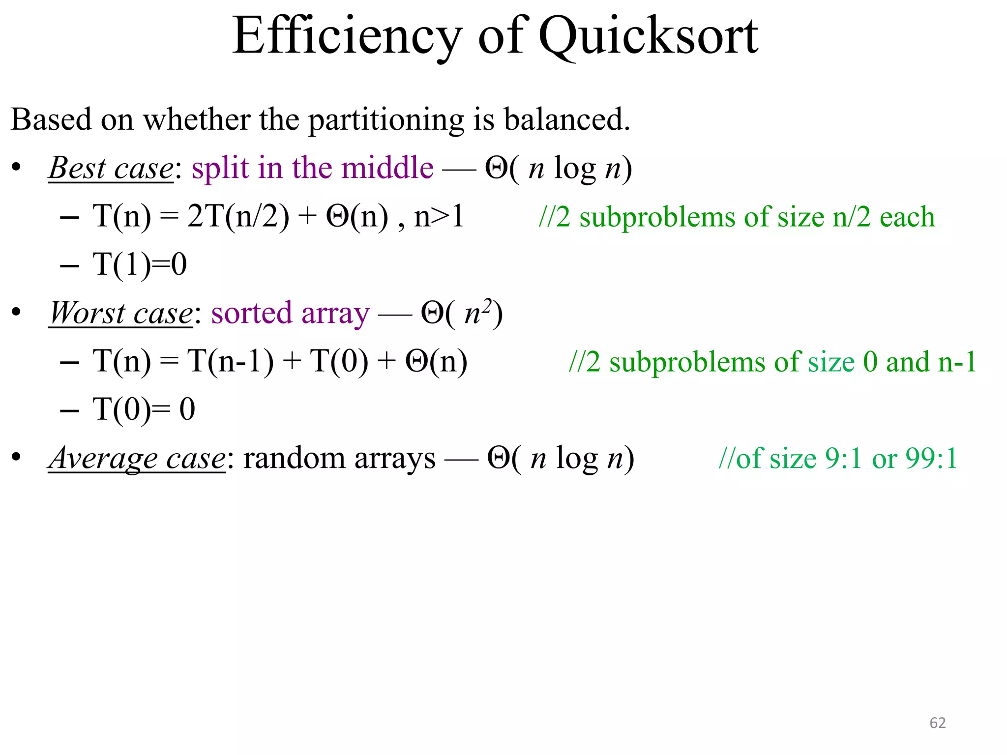

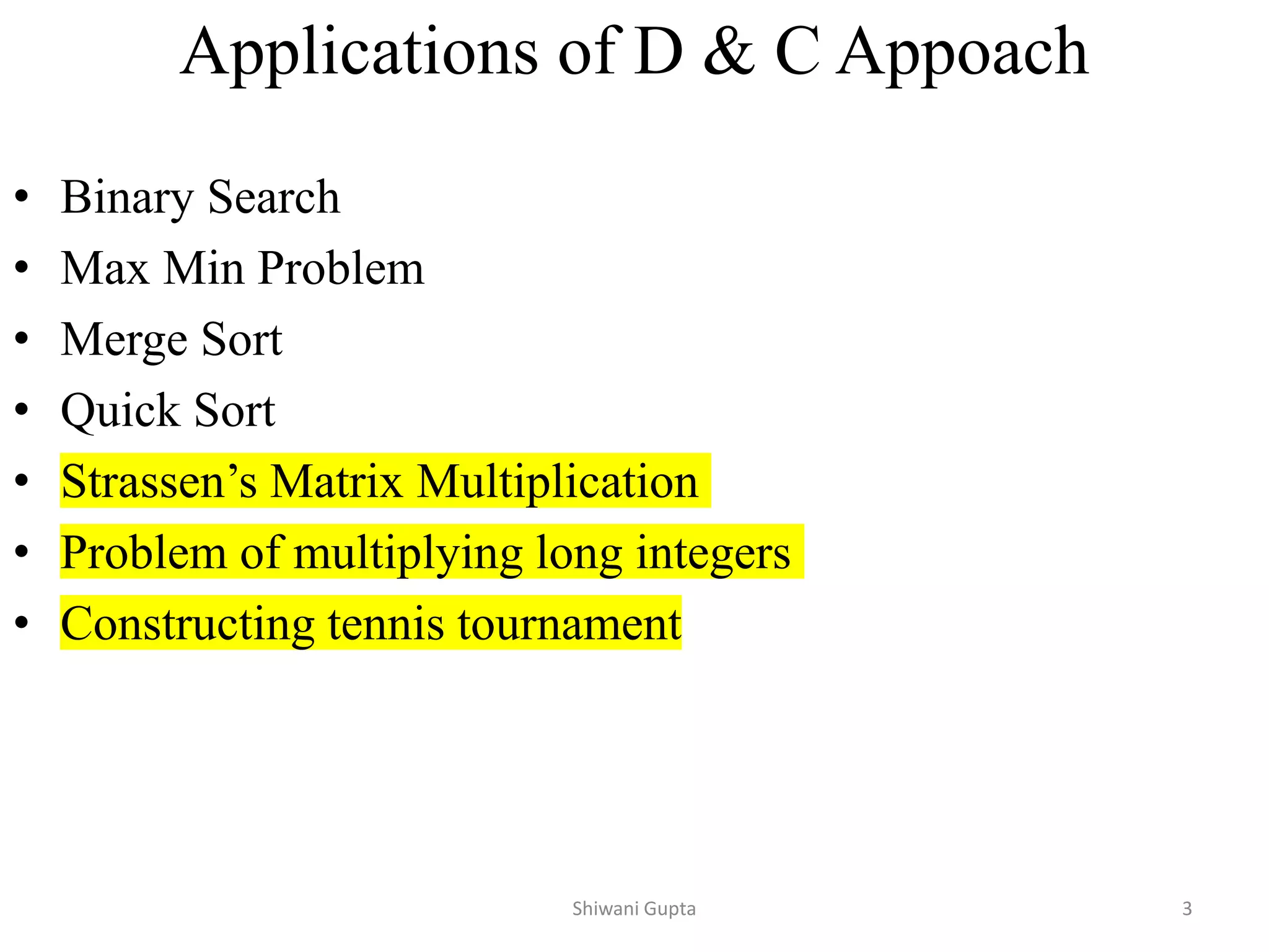
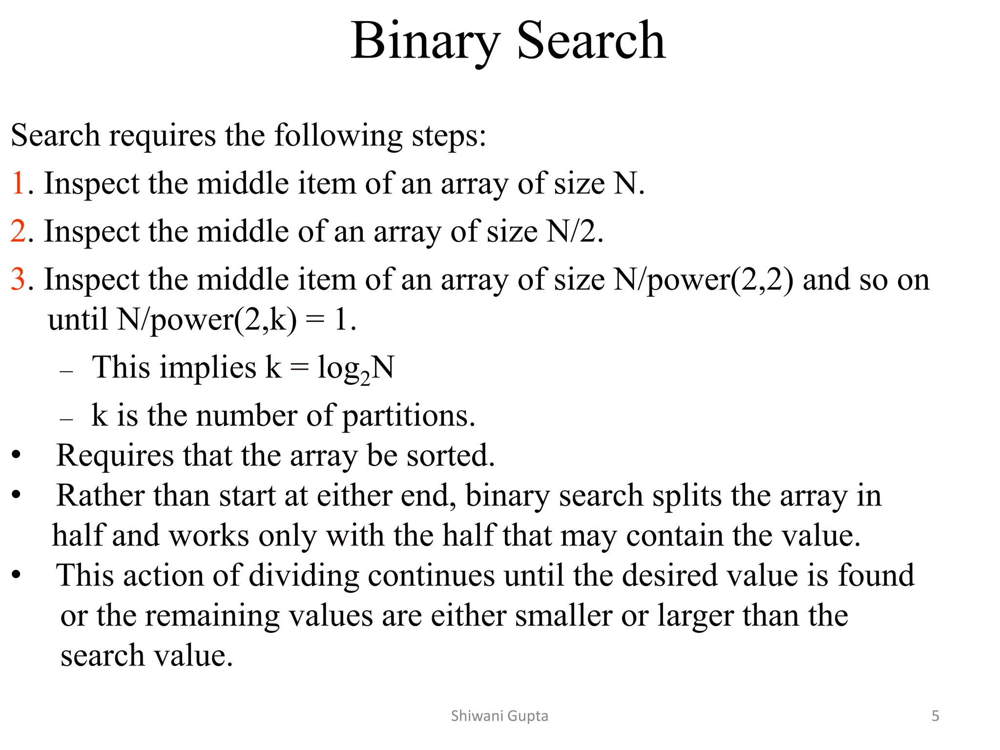
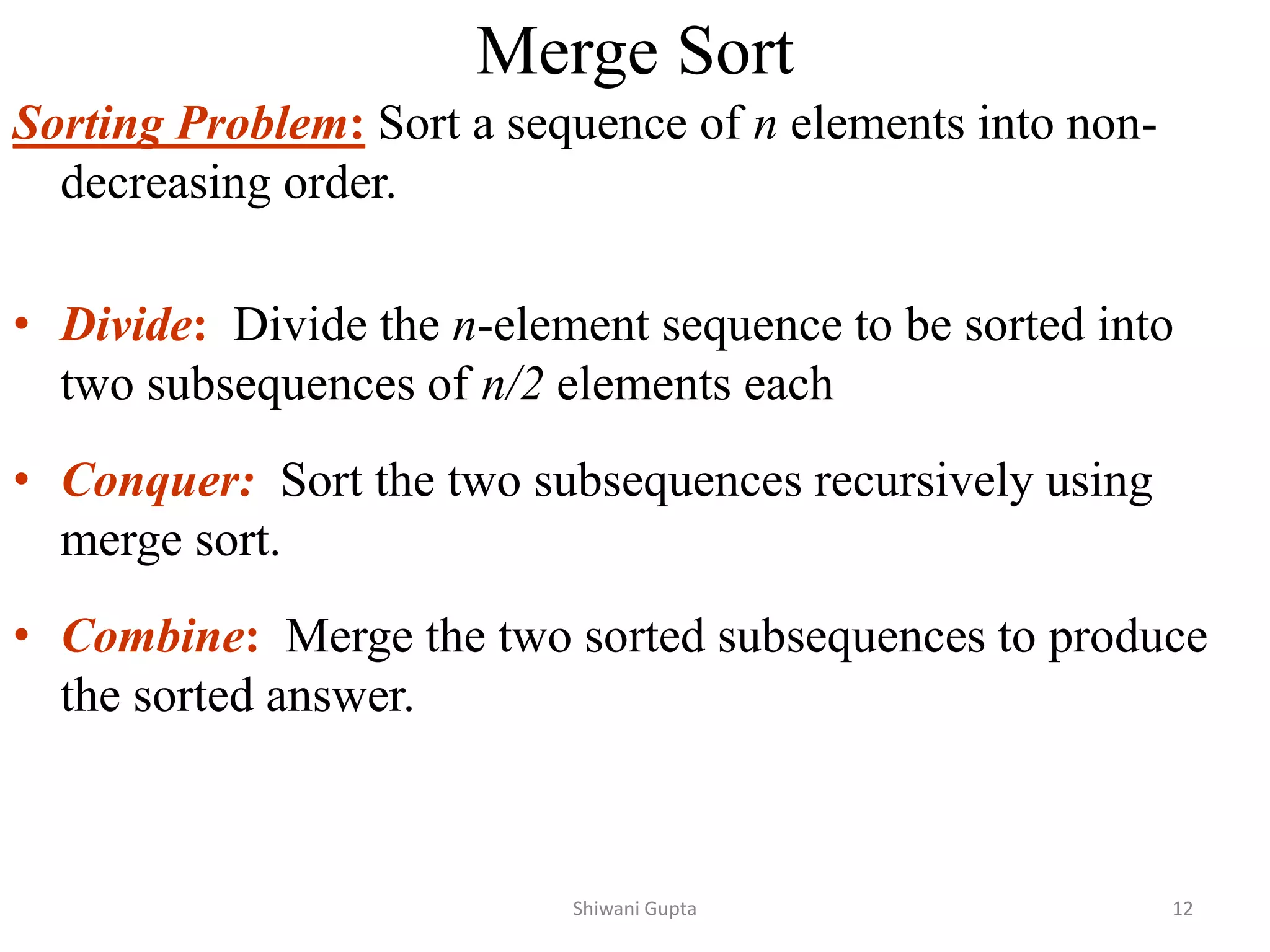
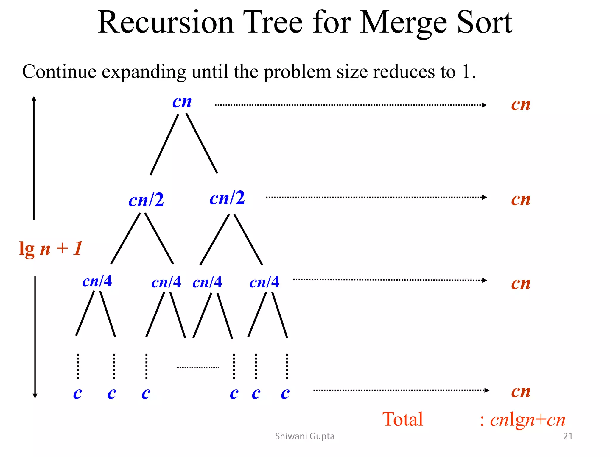
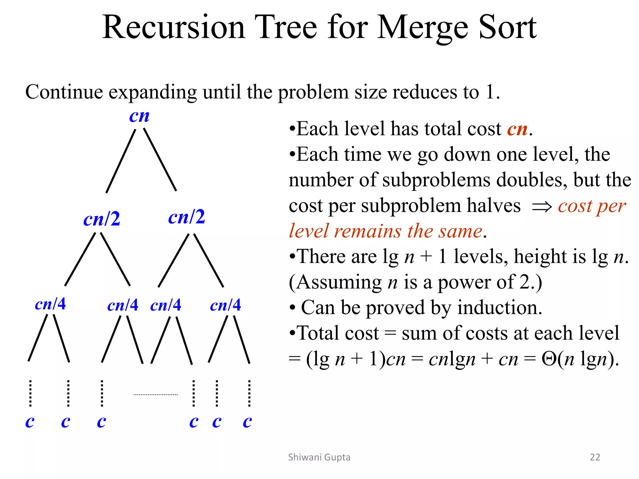
The document describes various divide and conquer algorithms including binary search, merge sort, quicksort, and finding maximum and minimum elements. It begins by explaining the general divide and conquer approach of dividing a problem into smaller subproblems, solving the subproblems independently, and combining the solutions. Several examples are then provided with pseudocode and analysis of their divide and conquer implementations. Key algorithms covered in the document include binary search (log n time), merge sort (n log n time), and quicksort (n log n time on average).


![UNIT V Searching Sorting Hashing Techniques [Autosaved].pptx](https://cdn.slidesharecdn.com/ss_thumbnails/unitvsearchingsortinghashingtechniquesautosaved-241126054304-95a69c51-thumbnail.jpg?width=600ounds&width=560&fit=bounds)
![UNIT V Searching Sorting Hashing Techniques [Autosaved].pptx](https://cdn.slidesharecdn.com/ss_thumbnails/unitvsearchingsortinghashingtechniquesautosaved-241014040608-74caa0f6-thumbnail.jpg?width=600ounds&width=560&fit=bounds)


